NumPy is a Python library that provides a simple yet powerful data structure: the n-dimensional array. This is the foundation on which almost all the power of Python’s data science toolkit is built, and learning NumPy is the first step on any Python data scientist’s journey. This tutorial will provide you with the knowledge you need to use NumPy and the higher-level libraries that rely on it.
In this tutorial you’ll learn:
- What core concepts in data science are made possible by NumPy
- How to create NumPy arrays using various methods
- How to manipulate NumPy arrays to perform useful calculations
- How to apply these new skills to real-world problems
To get the most out of this NumPy tutorial, you should be familiar with writing Python code. Working through the Introduction to Python learning path is a great way to make sure you’ve got the basic skills covered. If you’re familiar with matrix mathematics, then that will certainly be helpful as well. You don’t need to know anything about data science, however. You’ll learn that here.
There’s also a repository of NumPy code samples that you’ll see throughout this tutorial. You can use it for reference and experiment with the examples to see how changing the code changes the outcome. To download the code, click the link below:
Get Sample Code: Click here to get the sample code you’ll use to learn about NumPy in this tutorial.
Choosing NumPy: The Benefits
Since you already know Python, you may be asking yourself if you really have to learn a whole new paradigm to do data science. Python’s for loops are awesome! Reading and writing CSV files can be done with traditional code. However, there are some convincing arguments for learning a new paradigm.
Here are the top four benefits that NumPy can bring to your code:
- More speed: NumPy uses algorithms written in C that complete in nanoseconds rather than seconds.
- Fewer loops: NumPy helps you to reduce loops and keep from getting tangled up in iteration indices.
- Clearer code: Without loops, your code will look more like the equations you’re trying to calculate.
- Better quality: There are thousands of contributors working to keep NumPy fast, friendly, and bug free.
Because of these benefits, NumPy is the de facto standard for multidimensional arrays in Python data science, and many of the most popular libraries are built on top of it. Learning NumPy is a great way to set down a solid foundation as you expand your knowledge into more specific areas of data science.
Installing NumPy
It’s time to get everything set up so you can start learning how to work with NumPy. There are a few different ways to do this, and you can’t go wrong by following the instructions on the NumPy website. But there are some extra details to be aware of that are outlined below.
You’ll also be installing Matplotlib. You’ll use it in one of the later examples to explore how other libraries make use of NumPy.
Using Repl.it as an Online Editor
If you just want to get started with some examples, follow along with this tutorial, and start building some muscle memory with NumPy, then Repl.it is a great option for in-browser editing. You can sign up and fire up a Python environment in minutes. Along the left side, there’s a tab for packages. You can add as many as you want. For this NumPy tutorial, go with the current versions of NumPy and Matplotlib.
Here’s where you can find the packages in the interface:
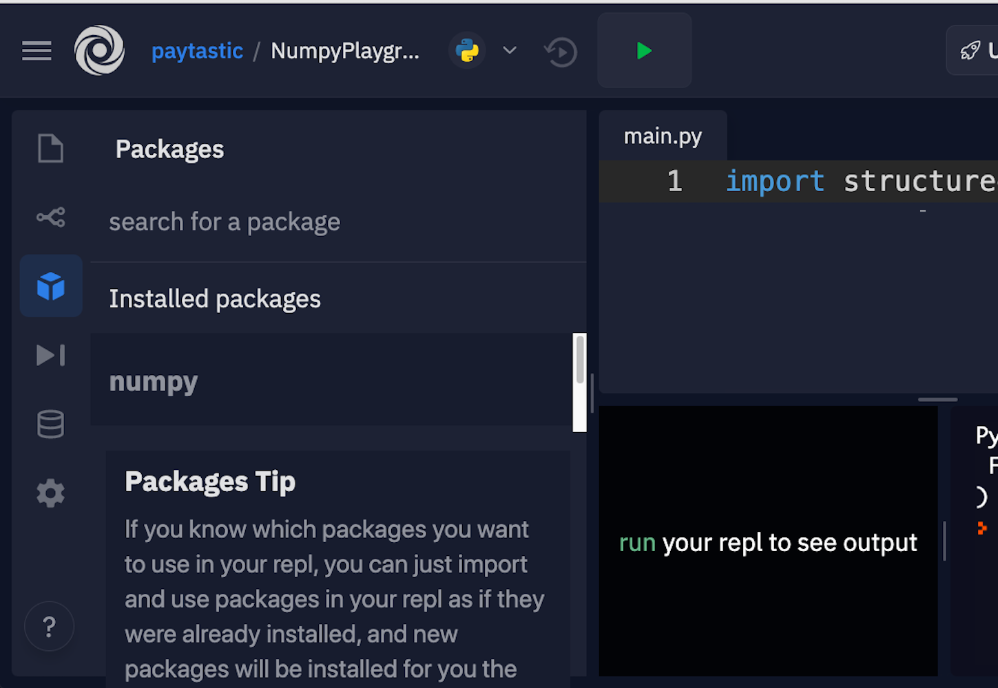
Luckily, they allow you to just click and install.
Installing NumPy With Anaconda
The Anaconda distribution is a suite of common Python data science tools bundled around a package manager that helps manage your virtual environments and project dependencies. It’s built around conda, which is the actual package manager. This is the method recommended by the NumPy project, especially if you’re stepping into data science in Python without having already set up a complex development environment.
If you’ve already got a workflow you like that uses pip, Pipenv, Poetry, or some other toolset, then it might be better not to add conda to the mix. The conda package repository is separate from PyPI, and conda itself sets up a separate little island of packages on your machine, so managing paths and remembering which package lives where can be a nightmare.
Once you’ve got conda installed, you can run the install command for the libraries you’ll need:
$ conda install numpy matplotlib
This will install what you need for this NumPy tutorial, and you’ll be all set to go.
Installing NumPy With pip
Although the NumPy project recommends using conda if you’re starting fresh, there’s nothing wrong with managing your environment yourself and just using good old pip, Pipenv, Poetry, or whatever other alternative to pip is your favorite.
Here are the commands to get set up with pip:
$ mkdir numpy-tutorial
$ cd numpy-tutorial
$ python3 -m venv .numpy-tutorial-venv
$ source .numpy-tutorial-venv/bin/activate

(.numpy-tutorial-venv)
$ pip install numpy matplotlib
Collecting numpy
  Downloading numpy-1.19.1-cp38-cp38-macosx_10_9_x86_64.whl (15.3 MB)
     |████████████████████████████████| 15.3 MB 2.7 MB/s
Collecting matplotlib
  Downloading matplotlib-3.3.0-1-cp38-cp38-macosx_10_9_x86_64.whl (11.4 MB)
     |████████████████████████████████| 11.4 MB 16.8 MB/s
...
After this, make sure your virtual environment is activated, and all your code should run as expected.
Using IPython, Notebooks, or JupyterLab
While the above sections should get you everything you need to get started, there are a couple more tools that you can optionally install to make working in data science more developer-friendly.
IPython is an upgraded Python read-eval-print loop (REPL) that makes editing code in a live interpreter session more straightforward and prettier. Here’s what an IPython REPL session looks like:
In [1]: import numpy as np

In [2]: digits = np.array([
   ...:     [1, 2, 3],
   ...:     [4, 5, 6],
   ...:     [6, 7, 9],
   ...: ])

In [3]: digits
Out[3]:
array([[1, 2, 3],
       [4, 5, 6],
       [6, 7, 9]])
It has several differences from a basic Python REPL, including its line numbers, use of colors, and quality of array visualizations. There are also a lot of user-experience bonuses that make it more pleasant to enter, re-enter, and edit code.
You can install IPython as a standalone:
$ pip install ipython
Alternatively, if you wait and install any of the subsequent tools, then they’ll include a copy of IPython.
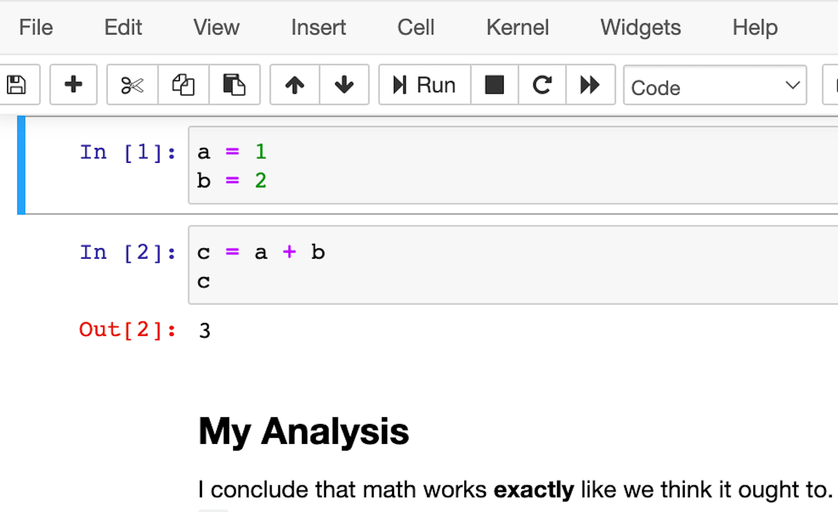
A slightly more featureful alternative to a REPL is a notebook. Notebooks are a slightly different style of writing Python than standard scripts, though. Instead of a traditional Python file, they give you a series of mini-scripts called cells that you can run and re-run in whatever order you want, all in the same Python memory session.
One neat thing about notebooks is that you can include graphs and render Markdown paragraphs between cells, so they’re really nice for writing up data analyses right inside the code!
Here’s what it looks like:
The most popular notebook offering is probably the Jupyter Notebook, but nteract is another option that wraps the Jupyter functionality and attempts to make it a bit more approachable and powerful.
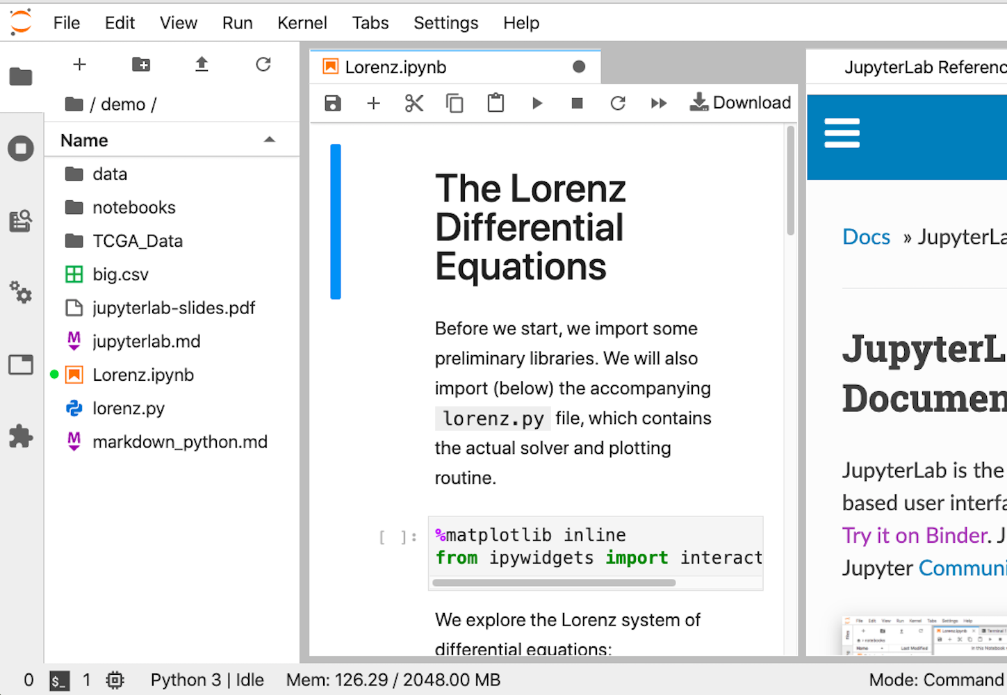
However, if you’re looking at Jupyter Notebook and thinking that it needs more IDE-like qualities, then JupyterLab is another option. You can customize text editors, notebooks, terminals, and custom components, all in a browser-based interface. It will likely be more comfortable for people coming from MatLab. It’s the youngest of the offerings, but its 1.0 release was back in 2019, so it should be stable and full featured.
This is what the interface looks like:
Whichever option you choose, once you have it installed, you’ll be ready to run your first lines of NumPy code. It’s time for the first example.
Hello NumPy: Curving Test Grades Tutorial
This first example introduces a few core concepts in NumPy that you’ll use throughout the rest of the tutorial:
- Creating arrays using
numpy.array() - Treating complete arrays like individual values to make vectorized calculations more readable
- Using built-in NumPy functions to modify and aggregate the data
These concepts are the core of using NumPy effectively.
The scenario is this: You’re a teacher who has just graded your students on a recent test. Unfortunately, you may have made the test too challenging, and most of the students did worse than expected. To help everybody out, you’re going to curve everyone’s grades.
It’ll be a relatively rudimentary curve, though. You’ll take whatever the average score is and declare that a C. Additionally, you’ll make sure that the curve doesn’t accidentally hurt your students’ grades or help so much that the student does better than 100%.
Enter this code into your REPL:
 1>>> import numpy as np
 2>>> CURVE_CENTER = 80
 3>>> grades = np.array([72, 35, 64, 88, 51, 90, 74, 12])
 4>>> def curve(grades):
 5...     average = grades.mean()
 6...     change = CURVE_CENTER - average
 7...     new_grades = grades + change
 8...     return np.clip(new_grades, grades, 100)
 9...
10>>> curve(grades)
11array([ 91.25,  54.25,  83.25, 100.  ,  70.25, 100.  ,  93.25,  31.25])
The original scores have been increased based on where they were in the pack, but none of them were pushed over 100%.
Here are the important highlights:
- Line 1 imports NumPy using the
npalias, which is a common convention that saves you a few keystrokes. - Line 3 creates your first NumPy array, which is one-dimensional and has a shape of
(8,)and a data type ofint64. Don’t worry too much about these details yet. You’ll explore them in more detail later in the tutorial. - Line 5 takes the average of all the scores using
.mean(). Arrays have a lot of methods.
On line 7, you take advantage of two important concepts at once:
- Vectorization
- Broadcasting
Vectorization is the process of performing the same operation in the same way for each element in an array. This removes for loops from your code but achieves the same result.
Broadcasting is the process of extending two arrays of different shapes and figuring out how to perform a vectorized calculation between them. Remember, grades is an array of numbers of shape (8,) and change is a scalar, or single number, essentially with shape (1,). In this case, NumPy adds the scalar to each item in the array and returns a new array with the results.
Finally, on line 8, you limit, or clip, the values to a set of minimums and maximums. In addition to array methods, NumPy also has a large number of built-in functions. You don’t need to memorize them all—that’s what documentation is for. Anytime you get stuck or feel like there should be an easier way to do something, take a peek at the documentation and see if there isn’t already a routine that does exactly what you need.
In this case, you need a function that takes an array and makes sure the values don’t exceed a given minimum or maximum. clip() does exactly that.
Line 8 also provides another example of broadcasting. For the second argument to clip(), you pass grades, ensuring that each newly curved grade doesn’t go lower than the original grade. But for the third argument, you pass a single value: 100. NumPy takes that value and broadcasts it against every element in new_grades, ensuring that none of the newly curved grades exceeds a perfect score.
Getting Into Shape: Array Shapes and Axes
Now that you’ve seen some of what NumPy can do, it’s time to firm up that foundation with some important theory. There are a few concepts that are important to keep in mind, especially as you work with arrays in higher dimensions.
Vectors, which are one-dimensional arrays of numbers, are the least complicated to keep track of. Two dimensions aren’t too bad, either, because they’re similar to spreadsheets. But things start to get tricky at three dimensions, and visualizing four? Forget about it.
Mastering Shape
Shape is a key concept when you’re using multidimensional arrays. At a certain point, it’s easier to forget about visualizing the shape of your data and to instead follow some mental rules and trust NumPy to tell you the correct shape.
All arrays have a property called .shape that returns a tuple of the size in each dimension. It’s less important which dimension is which, but it’s critical that the arrays you pass to functions are in the shape that the functions expect. A common way to confirm that your data has the proper shape is to print the data and its shape until you’re sure everything is working like you expect.
This next example will show this process. You’ll create an array with a complex shape, check it, and reorder it to look like it’s supposed to:
In [1]: import numpy as np

In [2]: temperatures = np.array([
   ...:     29.3, 42.1, 18.8, 16.1, 38.0, 12.5,
   ...:     12.6, 49.9, 38.6, 31.3, 9.2, 22.2
   ...: ]).reshape(2, 2, 3)

In [3]: temperatures.shape
Out[3]: (2, 2, 3)

In [4]: temperatures
Out[4]:
array([[[29.3, 42.1, 18.8],
        [16.1, 38. , 12.5]],

       [[12.6, 49.9, 38.6],
        [31.3,  9.2, 22.2]]])

In [5]: np.swapaxes(temperatures, 1, 2)
Out[5]:
array([[[29.3, 16.1],
        [42.1, 38. ],
        [18.8, 12.5]],

       [[12.6, 31.3],
        [49.9,  9.2],
        [38.6, 22.2]]])
Here, you use a numpy.ndarray method called .reshape() to form a 2 × 2 × 3 block of data. When you check the shape of your array in input 3, it’s exactly what you told it to be. However, you can see how printed arrays quickly become hard to visualize in three or more dimensions. After you swap axes with .swapaxes(), it becomes little clearer which dimension is which. You’ll see more about axes in the next section.
Shape will come up again in the section on broadcasting. For now, just keep in mind that these little checks don’t cost anything. You can always delete the cells or get rid of the code once things are running smoothly.
Understanding Axes
The example above shows how important it is to know not only what shape your data is in but also which data is in which axis. In NumPy arrays, axes are zero-indexed and identify which dimension is which. For example, a two-dimensional array has a vertical axis (axis 0) and a horizontal axis (axis 1). Lots of functions and commands in NumPy change their behavior based on which axis you tell them to process.
This example will show how .max() behaves by default, with no axis argument, and how it changes functionality depending on which axis you specify when you do supply an argument:
In [1]: import numpy as np

In [2]: table = np.array([
   ...:     [5, 3, 7, 1],
   ...:     [2, 6, 7 ,9],
   ...:     [1, 1, 1, 1],
   ...:     [4, 3, 2, 0],
   ...: ])

In [3]: table.max()
Out[3]: 9

In [4]: table.max(axis=0)
Out[4]: array([5, 6, 7, 9])

In [5]: table.max(axis=1)
Out[5]: array([7, 9, 1, 4])
By default, .max() returns the largest value in the entire array, no matter how many dimensions there are. However, once you specify an axis, it performs that calculation for each set of values along that particular axis. For example, with an argument of axis=0, .max() selects the maximum value in each of the four vertical sets of values in table and returns an array that has been flattened, or aggregated into a one-dimensional array.
In fact, many of NumPy’s functions behave this way: If no axis is specified, then they perform an operation on the entire dataset. Otherwise, they perform the operation in an axis-wise fashion.
Broadcasting
So far, you’ve seen a couple of smaller examples of broadcasting, but the topic will start to make more sense the more examples you see. Fundamentally, it functions around one rule: arrays can be broadcast against each other if their dimensions match or if one of the arrays has a size of 1.
If the arrays match in size along an axis, then elements will be operated on element-by-element, similar to how the built-in Python function zip() works. If one of the arrays has a size of 1 in an axis, then that value will be broadcast along that axis, or duplicated as many times as necessary to match the number of elements along that axis in the other array.
Here’s a quick example. Array A has the shape (4, 1, 8), and array B has the shape (1, 6, 8). Based on the rules above, you can operate on these arrays together:
- In axis 0,
Ahas a4andBhas a1, soBcan be broadcast along that axis. - In axis 1,
Ahas a 1 andBhas a 6, soAcan be broadcast along that axis. - In axis 2, the two arrays have matching sizes, so they can operate successfully.
All three axes successfully follow the rule.
You can set up the arrays like this:
In [1]: import numpy as np

In [2]: A = np.arange(32).reshape(4, 1, 8)

In [3]: A
Out[3]:
array([[[ 0,  1,  2,  3,  4,  5,  6,  7]],

       [[ 8,  9, 10, 11, 12, 13, 14, 15]],

       [[16, 17, 18, 19, 20, 21, 22, 23]],

       [[24, 25, 26, 27, 28, 29, 30, 31]]])

In [4]: B = np.arange(48).reshape(1, 6, 8)

In [5]: B
Out[5]:
array([[[ 0,  1,  2,  3,  4,  5,  6,  7],
        [ 8,  9, 10, 11, 12, 13, 14, 15],
        [16, 17, 18, 19, 20, 21, 22, 23],
        [24, 25, 26, 27, 28, 29, 30, 31],
        [32, 33, 34, 35, 36, 37, 38, 39],
        [40, 41, 42, 43, 44, 45, 46, 47]]])
A has 4 planes, each with 1 row and 8 columns. B has only 1 plane with 6 rows and 8 columns. Watch what NumPy does for you when you try to do a calculation between them!
Add the two arrays together:
In [7]: A + B
Out[7]:
array([[[ 0,  2,  4,  6,  8, 10, 12, 14],
        [ 8, 10, 12, 14, 16, 18, 20, 22],
        [16, 18, 20, 22, 24, 26, 28, 30],
        [24, 26, 28, 30, 32, 34, 36, 38],
        [32, 34, 36, 38, 40, 42, 44, 46],
        [40, 42, 44, 46, 48, 50, 52, 54]],

       [[ 8, 10, 12, 14, 16, 18, 20, 22],
        [16, 18, 20, 22, 24, 26, 28, 30],
        [24, 26, 28, 30, 32, 34, 36, 38],
        [32, 34, 36, 38, 40, 42, 44, 46],
        [40, 42, 44, 46, 48, 50, 52, 54],
        [48, 50, 52, 54, 56, 58, 60, 62]],

       [[16, 18, 20, 22, 24, 26, 28, 30],
        [24, 26, 28, 30, 32, 34, 36, 38],
        [32, 34, 36, 38, 40, 42, 44, 46],
        [40, 42, 44, 46, 48, 50, 52, 54],
        [48, 50, 52, 54, 56, 58, 60, 62],
        [56, 58, 60, 62, 64, 66, 68, 70]],

       [[24, 26, 28, 30, 32, 34, 36, 38],
        [32, 34, 36, 38, 40, 42, 44, 46],
        [40, 42, 44, 46, 48, 50, 52, 54],
        [48, 50, 52, 54, 56, 58, 60, 62],
        [56, 58, 60, 62, 64, 66, 68, 70],
        [64, 66, 68, 70, 72, 74, 76, 78]]])
The way broadcasting works is that NumPy duplicates the plane in B three times so that you have a total of four, matching the number of planes in A. It also duplicates the single row in A five times for a total of six, matching the number of rows in B. Then it adds each element in the newly expanded A array to its counterpart in the same location in B. The result of each calculation shows up in the corresponding location of the output.
Note: This is a good way to create an array from a range using arange()!
Once again, even though you can use words like “plane,” “row,” and “column” to describe how the shapes in this example are broadcast to create matching three-dimensional shapes, things get more complicated at higher dimensions. A lot of times, you’ll have to simply follow the broadcasting rules and do lots of print-outs to make sure things are working as planned.
Understanding broadcasting is an important part of mastering vectorized calculations, and vectorized calculations are the way to write clean, idiomatic NumPy code.
Data Science Operations: Filter, Order, Aggregate
That wraps up a section that was heavy in theory but a little light on practical, real-world examples. In this section, you’ll work through some examples of real, useful data science operations: filtering, sorting, and aggregating data.
Indexing
Indexing uses many of the same idioms that normal Python code uses. You can use positive or negative indices to index from the front or back of the array. You can use a colon (:) to specify “the rest” or “all,” and you can even use two colons to skip elements as with regular Python lists.
Here’s the difference: NumPy arrays use commas between axes, so you can index multiple axes in one set of square brackets. An example is the easiest way to show this off. It’s time to confirm Dürer’s magic square!
The number square below has some amazing properties. If you add up any of the rows, columns, or diagonals, then you’ll get the same number, 34. That’s also what you’ll get if you add up each of the four quadrants, the center four squares, the four corner squares, or the four corner squares of any of the contained 3 × 3 grids. You’re going to prove it!
Fun fact: In the bottom row, the numbers 15 and 14 are in the middle, representing the year that Dürer created this square. The numbers 1 and 4 are also in that row, representing the first and fourth letters of the alphabet, A and D, which are the initials of the square’s creator, Albrecht Dürer!
Enter the following into your REPL:
In [1]: import numpy as np

In [2]: square = np.array([
   ...:     [16, 3, 2, 13],
   ...:     [5, 10, 11, 8],
   ...:     [9, 6, 7, 12],
   ...:     [4, 15, 14, 1]
   ...: ])

In [3]: for i in range(4):
   ...:     assert square[:, i].sum() == 34
   ...:     assert square[i, :].sum() == 34
   ...:

In [4]: assert square[:2, :2].sum() == 34

In [5]: assert square[2:, :2].sum() == 34

In [6]: assert square[:2, 2:].sum() == 34

In [7]: assert square[2:, 2:].sum() == 34
Inside the for loop, you verify that all the rows and all the columns add up to 34. After that, using selective indexing, you verify that each of the quadrants also adds up to 34.
One last thing to note is that you’re able to take the sum of any array to add up all of its elements globally with square.sum(). This method can also take an axis argument to do an axis-wise summing instead.
Masking and Filtering
Index-based selection is great, but what if you want to filter your data based on more complicated nonuniform or nonsequential criteria? This is where the concept of a mask comes into play.
A mask is an array that has the exact same shape as your data, but instead of your values, it holds Boolean values: either True or False. You can use this mask array to index into your data array in nonlinear and complex ways. It will return all of the elements where the Boolean array has a True value.
Here’s an example showing the process, first in slow motion and then how it’s typically done, all in one line:
In [1]: import numpy as np

In [2]: numbers = np.linspace(5, 50, 24, dtype=int).reshape(4, -1)

In [3]: numbers
Out[3]:
array([[ 5, 6,  8, 10, 12, 14],
       [16, 18, 20, 22, 24, 26],
       [28, 30, 32, 34, 36, 38],
       [40, 42, 44, 46, 48, 50]])

In [4]: mask = numbers % 4 == 0

In [5]: mask
Out[5]:
array([[False, False,  True, False,  True, False],
       [ True, False,  True, False,  True, False],
       [ True, False,  True, False,  True, False],
       [ True, False,  True, False,  True, False]])

In [6]: numbers[mask]
Out[6]: array([ 8, 12, 16, 20, 24, 28, 32, 36, 40, 44, 48])

In [7]: by_four = numbers[numbers % 4 == 0]

In [8]: by_four
Out[8]: array([ 8, 12, 16, 20, 24, 28, 32, 36, 40, 44, 48])
You’ll see an explanation of the new array creation tricks in input 2 in a moment, but for now, focus on the meat of the example. These are the important parts:
- Input 4 creates the mask by performing a vectorized Boolean computation, taking each element and checking to see if it divides evenly by four. This returns a mask array of the same shape with the element-wise results of the computation.
- Input 6 uses this mask to index into the original
numbersarray. This causes the array to lose its original shape, reducing it to one dimension, but you still get the data you’re looking for. - Input 7 provides a more traditional, idiomatic masked selection that you might see in the wild, with an anonymous filtering array created inline, inside the selection brackets. This syntax is similar to usage in the R programming language.
Coming back to input 2, you encounter three new concepts:
- Using
np.linspace()to generate an evenly spaced array - Setting the
dtypeof an output - Reshaping an array with
-1
np.linspace() generates n numbers evenly distributed between a minimum and a maximum, which is useful for evenly distributed sampling in scientific plotting.
Because of the particular calculation in this example, it makes life easier to have integers in the numbers array. But because the space between 5 and 50 doesn’t divide evenly by 24, the resulting numbers would be floating-point numbers. You specify a dtype of int to force the function to round down and give you whole integers. You’ll see a more detailed discussion of data types later on.
Finally, array.reshape() can take -1 as one of its dimension sizes. That signifies that NumPy should just figure out how big that particular axis needs to be based on the size of the other axes. In this case, with 24 values and a size of 4 in axis 0, axis 1 ends up with a size of 6.
Here’s one more example to show off the power of masked filtering. The normal distribution is a probability distribution in which roughly 95.45% of values occur within two standard deviations of the mean.
You can verify that with a little help from NumPy’s random module for generating random values:
In [1]: import numpy as np

In [2]: from numpy.random import default_rng

In [3]: rng = default_rng()

In [4]: values = rng.standard_normal(10000)

In [5]: values[:5]
Out[5]: array([ .9779210858,  1.8361585253,  -.3641365235,
               -.1311344527, 1.286542056 ])

In [6]: std = values.std()

In [7]: std
Out[7]: .9940375551073492

In [8]: filtered = values[(values > -2 * std) & (values < 2 * std)]

In [9]: filtered.size
Out[9]: 9565

In [10]: values.size
Out[10]: 10000

In [11]: filtered.size / values.size
Out[11]: 0.9565
Here you use a potentially strange-looking syntax to combine filter conditions: a binary & operator. Why would that be the case? It’s because NumPy designates & and | as the vectorized, element-wise operators to combine Booleans. If you try to do A and B, then you’ll get a warning about how the truth value for an array is weird, because the and is operating on the truth value of the whole array, not element by element.
Transposing, Sorting, and Concatenating
Other manipulations, while not quite as common as indexing or filtering, can also be very handy depending on the situation you’re in. You’ll see a few examples in this section.
Here’s transposing an array:
In [1]: import numpy as np

In [2]: a = np.array([
   ...:     [1, 2],
   ...:     [3, 4],
   ...:     [5, 6],
   ...: ])

In [3]: a.T
Out[3]:
array([[1, 3, 5],
       [2, 4, 6]])

In [4]: a.transpose()
Out[4]:
array([[1, 3, 5],
       [2, 4, 6]])
When you calculate the transpose of an array, the row and column indices of every element are switched. Item [0, 2], for example, becomes item [2, 0]. You can also use a.T as an alias for a.transpose().
The following code block shows sorting, but you’ll also see a more powerful sorting technique in the coming section on structured data:
In [1]: import numpy as np

In [2]: data = np.array([
   ...:     [7, 1, 4],
   ...:     [8, 6, 5],
   ...:     [1, 2, 3]
   ...: ])

In [3]: np.sort(data)
Out[3]:
array([[1, 4, 7],
       [5, 6, 8],
       [1, 2, 3]])

In [4]: np.sort(data, axis=None)
Out[4]: array([1, 1, 2, 3, 4, 5, 6, 7, 8])

In [5]: np.sort(data, axis=0)
Out[5]:
array([[1, 1, 3],
       [7, 2, 4],
       [8, 6, 5]])
Omitting the axis argument automatically selects the last and innermost dimension, which is the rows in this example. Using None flattens the array and performs a global sort. Otherwise, you can specify which axis you want. In output 5, each column of the array still has all of its elements but they have been sorted low-to-high inside that column.
Finally, here’s an example of concatenation. While there’s a np.concatenate() function, there are also a number of helper functions that are sometimes easier to read.
Here are some examples:
In [1]: import numpy as np

In [2]: a = np.array([
   ...:     [4, 8],
   ...:     [6, 1]
   ...: ])

In [3]: b = np.array([
   ...:     [3, 5],
   ...:     [7, 2],
   ...: ])

In [4]: np.hstack((a, b))
Out[4]:
array([[4, 8, 3, 5],
       [6, 1, 7, 2]])

In [5]: np.vstack((b, a))
Out[5]:
array([[3, 5],
       [7, 2],
       [4, 8],
       [6, 1]])

In [6]: np.concatenate((a, b))
Out[6]:
array([[4, 8],
       [6, 1],
       [3, 5],
       [7, 2]])

In [7]: np.concatenate((a, b), axis=None)
Out[7]: array([4, 8, 6, 1, 3, 5, 7, 2])
Inputs 4 and 5 show the slightly more intuitive functions hstack() and vstack(). Inputs 6 and 7 show the more generic concatenate(), first without an axis argument and then with axis=None. This flattening behavior is similar in form to what you just saw with sort().
One important stumbling block to note is that all these functions take a tuple of arrays as their first argument rather than a variable number of arguments as you might expect. You can tell because there’s an extra pair of parentheses.
Aggregating
Your last stop on this tour of functionality before diving into some more advanced topics and examples is aggregation. You’ve already seen quite a few aggregating methods, including .sum(), .max(), .mean(), and .std(). You can reference NumPy’s larger library of functions to see more. Many of the mathematical, financial, and statistical functions use aggregation to help you reduce the number of dimensions in your data.
Practical Example 1: Implementing a Maclaurin Series
Now it’s time to see a realistic use case for the skills introduced in the sections above: implementing an equation.
One of the hardest things about converting mathematical equations to code without NumPy is that many of the visual similarities are missing, which makes it hard to tell what portion of the equation you’re looking at as you read the code. Summations are converted to more verbose for loops, and limit optimizations end up looking like while loops.
Using NumPy allows you to keep closer to a one-to-one representation from equation to code.
In this next example, you’ll encode the Maclaurin series for ex. Maclaurin series are a way of approximating more complicated functions with an infinite series of summed terms centered about zero.
For ex, the Maclaurin series is the following summation:

You add up terms starting at zero and going theoretically to infinity. Each nth term will be x raised to n and divided by n!, which is the notation for the factorial operation.
Now it’s time for you to put that into NumPy code. Create a file called maclaurin.py:
from math import e, factorial

import numpy as np

fac = np.vectorize(factorial)

def e_x(x, terms=10):
    """Approximates e^x using a given number of terms of
    the Maclaurin series
    """
    n = np.arange(terms)
    return np.sum((x ** n) / fac(n))

if __name__ == "__main__":
    print("Actual:", e ** 3)  # Using e from the standard library

    print("N (terms)\tMaclaurin\tError")

    for n in range(1, 14):
        maclaurin = e_x(3, terms=n)
        print(f"{n}\t\t{maclaurin:.03f}\t\t{e**3 - maclaurin:.03f}")
When you run this, you should see the following result:
$ python3 maclaurin.py
Actual: 20.085536923187664
N (terms) Maclaurin Error
1         1.000     19.086
2         4.000     16.086
3         8.500     11.586
4        13.000      7.086
5        16.375      3.711
6        18.400      1.686
7        19.412      0.673
8        19.846      0.239
9        20.009      0.076
10       20.063      0.022
11       20.080      0.006
12       20.084      0.001
13       20.085      0.000
As you increase the number of terms, your Maclaurin value gets closer and closer to the actual value, and your error shrinks smaller and smaller.
The calculation of each term involves taking x to the n power and dividing by n!, or the factorial of n. Adding, summing, and raising to powers are all operations that NumPy can vectorize automatically and quickly, but not so for factorial().
To use factorial() in a vectorized calculation, you have to use np.vectorize() to create a vectorized version. The documentation for np.vectorize() states that it’s little more than a thin wrapper that applies a for loop to a given function. There are no real performance benefits from using it instead of normal Python code, and there are potentially some overhead penalties. However, as you’ll see in a moment, the readability benefits are huge.
Once your vectorized factorial is in place, the actual code to calculate the entire Maclaurin series is shockingly short. It’s also readable. Most importantly, it’s almost exactly one-to-one with how the mathematical equation looks:
n = np.arange(terms)
return np.sum((x ** n) / fac(n))
This is such an important idea that it deserves to be repeated. With the exception of the extra line to initialize n, the code reads almost exactly the same as the original math equation. No for loops, no temporary i, j, k variables. Just plain, clear, math.
Just like that, you’re using NumPy for mathematical programming! For extra practice, try picking one of the other Maclaurin series and implementing it in a similar way.
Optimizing Storage: Data Types
Now that you have a bit more practical experience, it’s time to go back to theory and look at data types. Data types don’t play a central role in a lot of Python code. Numbers work like they’re supposed to, strings do other things, Booleans are true or false, and other than that, you make your own objects and collections.
In NumPy, though, there’s a little more detail that needs to be covered. NumPy uses C code under the hood to optimize performance, and it can’t do that unless all the items in an array are of the same type. That doesn’t just mean the same Python type. They have to be the same underlying C type, with the same shape and size in bits!
Numerical Types: int, bool, float, and complex
Since most of your data science and numerical calculations will tend to involve numbers, they seem like the best place to start. There are essentially four numerical types in NumPy code, and each one can take a few different sizes.
The table below breaks down the details of these types:
| Name | # of Bits | Python Type | NumPy Type |
|---|---|---|---|
| Integer | 64 | int |
np.int_ |
| Booleans | 8 | bool |
np.bool_ |
| Float | 64 | float |
np.float_ |
| Complex | 128 | complex |
np.complex_ |
These are just the types that map to existing Python types. NumPy also has types for the smaller-sized versions of each, like 8-, 16-, and 32-bit integers, 32-bit single-precision floating-point numbers, and 64-bit single-precision complex numbers. The documentation lists them in their entirety.
To specify the type when creating an array, you can provide a dtype argument:
In [1]: import numpy as np

In [2]: a = np.array([1, 3, 5.5, 7.7, 9.2], dtype=np.single)

In [3]: a
Out[3]: array([1. , 3. , 5.5, 7.7, 9.2], dtype=float32)

In [4]: b = np.array([1, 3, 5.5, 7.7, 9.2], dtype=np.uint8)

In [5]: b
Out[5]: array([1, 3, 5, 7, 9], dtype=uint8)
NumPy automatically converts your platform-independent type np.single to whatever fixed-size type your platform supports for that size. In this case, it uses np.float32. If your provided values don’t match the shape of the dtype you provided, then NumPy will either fix it for you or raise an error.
String Types: Sized Unicode
Strings behave a little strangely in NumPy code because NumPy needs to know how many bytes to expect, which isn’t usually a factor in Python programming. Luckily, NumPy does a pretty good job at taking care of less complex cases for you:
In [1]: import numpy as np

In [2]: names = np.array(["bob", "amy", "han"], dtype=str)

In [3]: names
Out[3]: array(['bob', 'amy', 'han'], dtype='<U3')

In [4]: names.itemsize
Out[4]: 12

In [5]: names = np.array(["bob", "amy", "han"])

In [6]: names
Out[6]: array(['bob', 'amy', 'han'], dtype='<U3')

In [7]: more_names = np.array(["bobo", "jehosephat"])

In [8]: np.concatenate((names, more_names))
Out[8]: array(['bob', 'amy', 'han', 'bobo', 'jehosephat'], dtype='<U10')
In input 2, you provide a dtype of Python’s built-in str type, but in output 3, it’s been converted into a little-endian Unicode string of size 3. When you check the size of a given item in input 4, you see that they’re each 12 bytes: three 4-byte Unicode characters.
Note: When dealing with NumPy data types, you have to think about things like the endianness of your values. In this case, the dtype '<U3' means that each value is the size of three Unicode characters, with the least-significant byte stored first in memory and the most-significant byte stored last. A dtype of '>U3' would signify the reverse.
As an example, NumPy represents the Unicode character “🐍” with the bytes 0xF4 0x01 0x00 with a dtype of '<U1' and 0x00 0x01 0xF4 with a dtype of '>U1'. Try it out by creating an array full of emoji, setting the dtype to one or the other, and then calling .tobytes() on your array!
If you’d like to study up on how Python treats the ones and zeros of your normal Python data types, then the official documentation for the struct library, which is a standard library module that works with raw bytes, is another good resource.
When you combine that with an array that has a larger item to create a new array in input 8, NumPy helpfully figures out how big the new array’s items need to be and grows them all to size <U10.
But here’s what happens when you try to modify one of the slots with a value larger than the capacity of the dtype:
In [9]: names[2] = "jamima"

In [10]: names
Out[10]: array(['bob', 'amy', 'jam'], dtype='<U3')
It doesn’t work as expected and truncates your value instead. If you already have an array, then NumPy’s automatic size detection won’t work for you. You get three characters and that’s it. The rest get lost in the void.
This is all to say that, in general, NumPy has your back when you’re working with strings, but you should always keep an eye on the size of your elements and make sure you have enough space when modifying or changing arrays in place.
Structured Arrays
Originally, you learned that array items all have to be the same data type, but that wasn’t entirely correct. NumPy has a special kind of array, called a record array or structured array, with which you can specify a type and, optionally, a name on a per-column basis. This makes sorting and filtering even more powerful, and it can feel similar to working with data in Excel, CSVs, or relational databases.
Here’s a quick example to show them off a little:
In [1]: import numpy as np

In [2]: data = np.array([
   ...:     ("joe", 32, 6),
   ...:     ("mary", 15, 20),
   ...:     ("felipe", 80, 100),
   ...:     ("beyonce", 38, 9001),
   ...: ], dtype=[("name", str, 10), ("age", int), ("power", int)])

In [3]: data[0]
Out[3]: ('joe', 32, 6)

In [4]: data["name"]
Out[4]: array(['joe', 'mary', 'felipe', 'beyonce'], dtype='<U10')

In [5]: data[data["power"] > 9000]["name"]
Out[5]: array(['beyonce'], dtype='<U10')
In input 2, you create an array, except each item is a tuple with a name, an age, and a power level. For the dtype, you actually provide a list of tuples with the information about each field: name is a 10-character Unicode field, and both age and power are standard 4-byte or 8-byte integers.
In input 3, you can see that the rows, known as records, are still accessible using the index.
In input 4, you see a new syntax for accessing an entire column, or field.
Finally, in input 5, you see a super-powerful combination of mask-based filtering based on a field and field-based selection. Notice how it’s not that much different to read the following SQL query:
SELECT name FROM data
WHERE power > 9000;
In both cases, the result is a list of names where the power level is over 9000.
You can even add in ORDER BY functionality by making use of np.sort():
In [6]: np.sort(data[data["age"] > 20], order="power")["name"]
Out[6]: array(['joe', 'felipe', 'beyonce'], dtype='<U10')
This sorts the data by power before retrieving it, which rounds out your selection of NumPy tools for selecting, filtering, and sorting items just like you might in SQL!
More on Data Types
This section of the tutorial was designed to get you just enough knowledge to be productive with NumPy’s data types, understand a little of how things work under the hood, and recognize some common pitfalls. It’s certainly not an exhaustive guide. The NumPy documentation on ndarrays has tons more resources.
There’s also a lot more information on dtype objects, including the different ways to construct, customize, and optimize them and how to make them more robust for all your data-handling needs. If you run into trouble and your data isn’t loading into arrays exactly how you expected, then that’s a good place to start.
Lastly, the NumPy recarray is a powerful object in its own right, and you’ve really only scratched the surface of the capabilities of structured datasets. It’s definitely worth reading through the recarray documentation as well as the documentation for the other specialized array subclasses that NumPy provides.
Looking Ahead: More Powerful Libraries
In this next section, you’ll move on to the powerhouse tools that are built on top of the foundational building blocks you saw above. Here are a few of the libraries that you’ll want to take a look at as your next steps on the road to total Python data science mastery.
pandas
pandas is a library that takes the concept of structured arrays and builds it out with tons of convenience methods, developer-experience improvements, and better automation. If you need to import data from basically anywhere, clean it, reshape it, polish it, and then export it into basically any format, then pandas is the library for you. It’s likely that at some point, you’ll import pandas as pd at the same time you import numpy as np.
The pandas documentation has a speedy tutorial filled with concrete examples called 10 Minutes to pandas. It’s a great resource that you can use to get some quick, hands-on practice.
scikit-learn
If your goals lie more in the direction of machine learning, then scikit-learn is the next step. Given enough data, you can do classification, regression, clustering, and more in just a few lines.
If you’re already comfortable with the math, then the scikit-learn documentation has a great list of tutorials to get you up and running in Python. If not, then the Math for Data Science Learning Path is a good place to start. Additionally, there’s also an entire learning path for machine learning.
It’s important for you to understand at least the basics of the mathematics behind the algorithms rather than just importing them and running with it. Bias in machine learning models is a huge ethical, social, and political issue.
Throwing data at models without a considering how to address the bias is a great way to get into trouble and negatively impact people’s lives. Doing some research and learning how to predict where bias might occur is a good start in the right direction.
Matplotlib
No matter what you’re doing with your data, at some point you’ll need to communicate your results to other humans, and Matplotlib is one of the main libraries for making that happen. For an introduction, check out Plotting with Matplotlib. In the next section, you’ll get some hands-on practice with Matplotlib, but you’ll use it for image manipulation rather than for making plots.
Practical Example 2: Manipulating Images With Matplotlib
It’s always neat when you’re working with a Python library and it hands you something that turns out to be a basic NumPy array. In this example, you’ll experience that in all its glory.
You’re going to load an image using Matplotlib, realize that RGB images are really just width × height × 3 arrays of int8 integers, manipulate those bytes, and use Matplotlib again to save that modified image once you’re done.
Download this image to work with:

It’s a picture of an adorable kitten that is 1920 pixels by 1299 pixels. You’re going to change the colors of those pixels.
Create a Python file called image_mod.py, then set up your imports and load the image:
 1import numpy as np
 2import matplotlib.image as mpimg
 3
 4img = mpimg.imread("kitty.jpg")
 5print(type(img))
 6print(img.shape)
This is a good start. Matplotlib has its own module for handling images, and you’re going to lean on that because it makes straightforward to read and write image formats.
If you run this code, then your friend the NumPy array will appear in the output:
$ python3 image_mod.py
<class 'numpy.ndarray'>
(1299, 1920, 3)
It’s an image with a height of 1299 pixels, a width of 1920 pixels, and three channels: one each for the red, green, and blue (RGB) color levels.
Want to see what happens when you drop out the R and G channels? Add this to your script:
 7output = img.copy()  # The original image is read-only!
 8output[:, :, :2] = 0
 9mpimg.imsave("blue.jpg", output)
Run it again and check the folder. There should be a new image:

Is your mind blown yet? Do you feel the power? Images are just fancy arrays! Pixels are just numbers!
But now, it’s time to do something a little more useful. You’re going to convert this image to grayscale. However, converting to grayscale is more complicated. Averaging the R, G, and B channels and making them all the same will give you an image that’s grayscale. But the human brain is weird, and that conversion doesn’t seem to handle the luminosity of the colors quite right.
In fact, it’s better to see it for yourself. You can use the fact that if you output an array with only one channel instead of three, then you can specify a color map, known as a cmap in the Matplotlib world. If you specify a cmap, then Matplotlib will handle the linear gradient calculations for you.
Get rid of the last three lines in your script and replace them with this:
 7averages = img.mean(axis=2)  # Take the average of each R, G, and B
 8mpimg.imsave("bad-gray.jpg", averages, cmap="gray")
These new lines create a new array called averages, which is a copy of the img array that you’ve flattened along axis 2 by taking the average of all three channels. You’ve averaged all three channels and outputted something with R, G, and B values equal to that average. When R, G, and B are all the same, the resulting color is on the grayscale.
What it ends up yielding isn’t terrible:

But you can do better using the luminosity method. This technique does a weighted average of the three channels, with the mindset that the color green drives how bright an image appears to be, and blue can make it appear darker. You’ll use the @ operator, which is NumPy’s operator for doing a traditional two-dimensional array dot product.
Replace those last two lines in your script again:
 7weights = np.array([0.3, 0.59, 0.11])
 8grayscale = img @ weights
 9mpimg.imsave("good-gray.jpg", grayscale, cmap="gray")
This time, instead of doing a flat average, you’re completing a dot product, which is a sort of weighted combination of the three values. Since the weights add up to one, it’s exactly equivalent to doing a weighted average of the three color channels.
Here’s the result:

The first image is a bit darker, and the edges and shadows are bolder. The second image is lighter and brighter, and the dark lines aren’t quite as bold. There you have it—you used Matplotlib and NumPy arrays to manipulate an image!
Conclusion
No matter how many dimensions your data lives in, NumPy gives you the tools to work with it. You can store it, reshape it, combine it, filter it, and sort it, and your code will read like you’re operating on only one number at a time rather than hundreds or thousands.
In this tutorial, you learned:
- The core concepts of data science made possible by NumPy
- How to create NumPy arrays using various methods
- How to manipulate NumPy arrays to perform useful calculations
- How to apply these new skills to real-world problems
Don’t forget to check out the repository of NumPy code samples from throughout this tutorial. You can use it for reference and experiment with the examples to see how changing the code changes the outcome:
Get Sample Code: Click here to get the sample code you’ll use to learn about NumPy in this tutorial.
Now you’re ready for the next steps in your data science journey. Whether you’re cleaning data, training neural networks, communicating using powerful plots, or aggregating data from the Internet of Things, these activities all start from the same place: the humble NumPy array.