Hugging Face Transformers: Leverage Open-Source AI in Python

Exploring Hugging Face

Hugging Face is a hub for state-of-the-art AI models. It’s primarily known for its wide range of open-source transformer-based models that excel in natural language processing (NLP), computer vision, and audio tasks. The platform offers several resources and services that cater to developers, researchers, businesses, and anyone interested in exploring AI models for their own use cases.

There’s a lot you can do with Hugging Face, but the primary offerings can be broken down into a few categories:

• Models: Hugging Face hosts a vast repository of pretrained AI models that are readily accessible and highly customizable. This repository is called the Model Hub, and it hosts models covering a wide range of tasks, including text classification, text generation, translation, summarization, speech recognition, image classification, and more. The platform is community-driven and allows users to contribute their own models, which facilitates a diverse and ever-growing selection.

• Datasets: Hugging Face has a library of thousands of datasets that you can use to train, benchmark, and enhance your models. These range from small-scale benchmarks to massive, real-world datasets that encompass a variety of domains, such as text, image, and audio data. Like the Model Hub, 🤗 Datasets supports community contributions and provides the tools you need to search, download, and use data in your machine learning projects.

• Spaces: Spaces allows you to deploy and share machine learning applications directly on the Hugging Face website. This service supports a variety of frameworks and interfaces, including Streamlit, Gradio, and Jupyter notebooks. It is particularly useful for showcasing model capabilities, hosting interactive demos, or for educational purposes, as it allows you to interact with models in real time.

• Paid offerings: Hugging Face also offers several paid services for enterprises and advanced users. These include the Pro Account, the Enterprise Hub, and Inference Endpoints. These solutions offer private model hosting, advanced collaboration tools, and dedicated support to help organizations scale their AI operations effectively.

These resources empower you to accelerate your AI projects and encourage collaboration and innovation within the community. Whether you’re a novice looking to experiment with pretrained models, or an enterprise seeking robust AI solutions, Hugging Face offers tools and platforms that cater to a wide range of needs.

This tutorial focuses on Transformers, a Python library that lets you run just about any model in the Model Hub. Before using transformers, you’ll need to understand what model cards are, and that’s what you’ll do next.

Understanding Model Cards

Model cards are the core components of the Model Hub, and you’ll need to understand how to search and read them to use models in Transformers. Model cards are nothing more than files that accompany each model to provide useful information. You can search for the model card you’re looking for on the Models page:

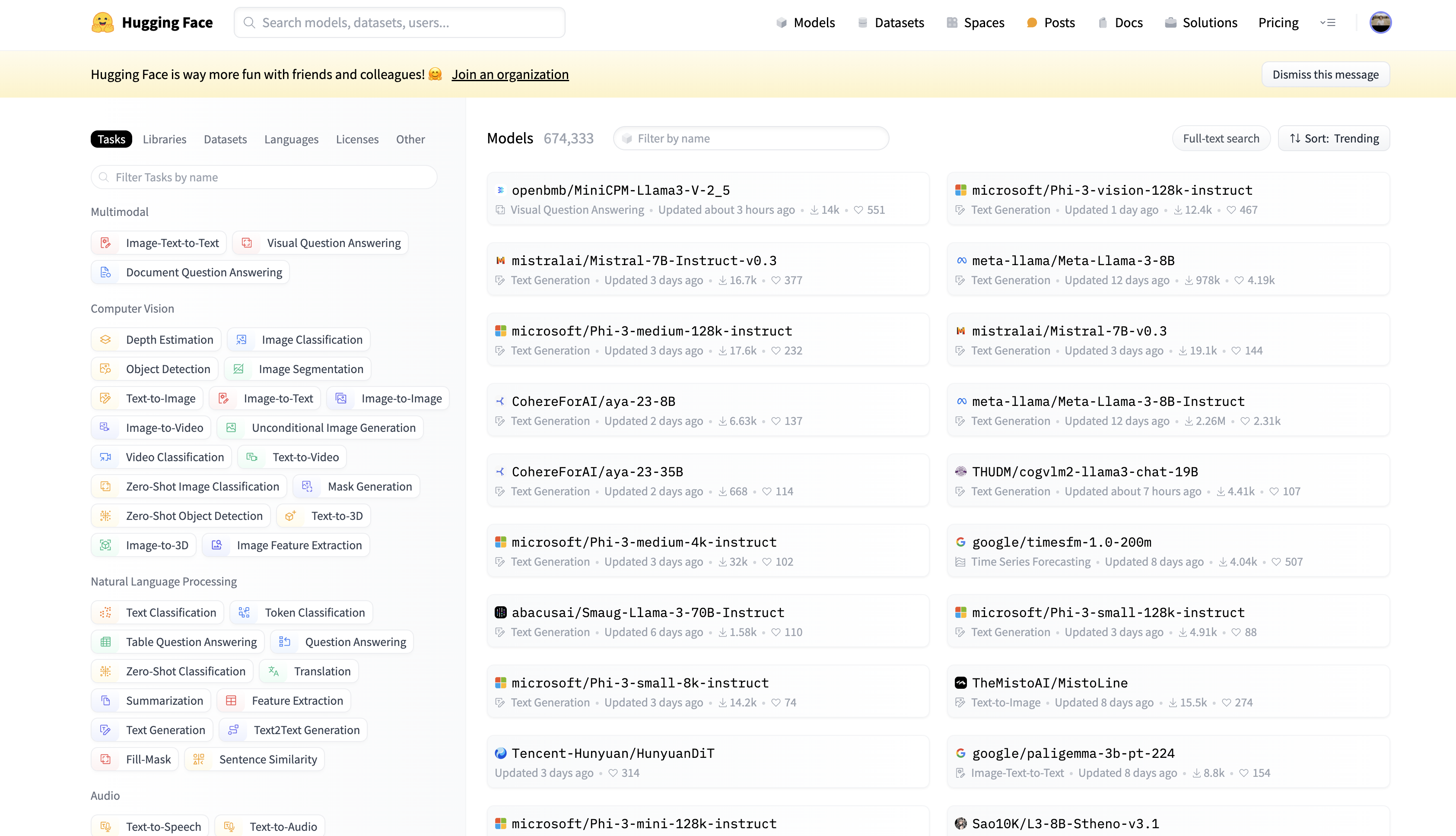
On the left side of the Models page, you can search for model cards based on the task you’re interested in. For example, if you’re interested in zero-shot text classification, you can click the Zero-Shot Classification button under the Natural Language Processing section:

In this search, you can see 266 different zero-shot text classification models, which is a paradigm where language models assign labels to text without explicit training or seeing any examples. In the upper-right corner, you can sort the search results based on model likes, downloads, creation dates, updated dates, and popularity trends.

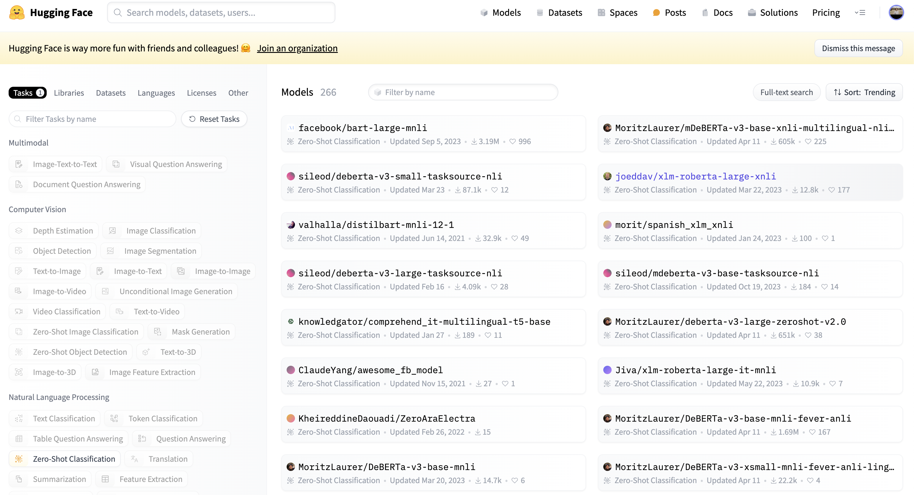
Each model card button tells you the model’s task, when it was last updated, and how many downloads and likes it has. When you click a model card button, say the one for the facebook/bart-large-mnli model, the model card will open and display all of the model’s information:

Even though a model card can display just about anything, Hugging Face has outlined the information that a good model card should provide. This includes detailed information about the model, its uses and limitations, the training parameters and experiment details, the dataset used to train the model, and the model’s evaluation performance.

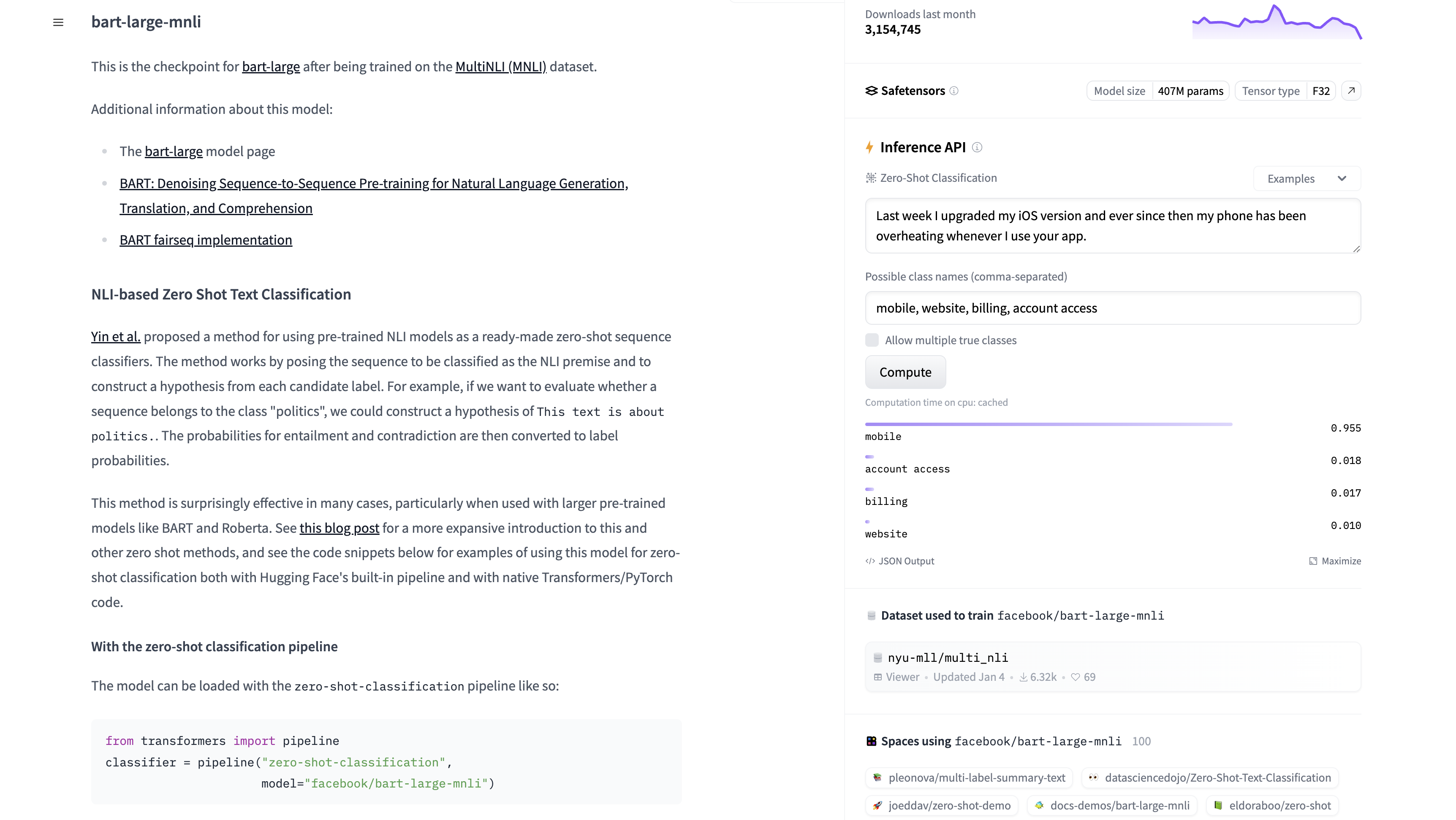
A high-quality model card also includes metadata such as the model’s license, references to the training data, and links to research papers that describe the model in detail. In some model cards, you’ll also get to tinker with a deployed instance of the model via the Inference API. You can see an example of this in the facebook/bart-large-mnli model card:

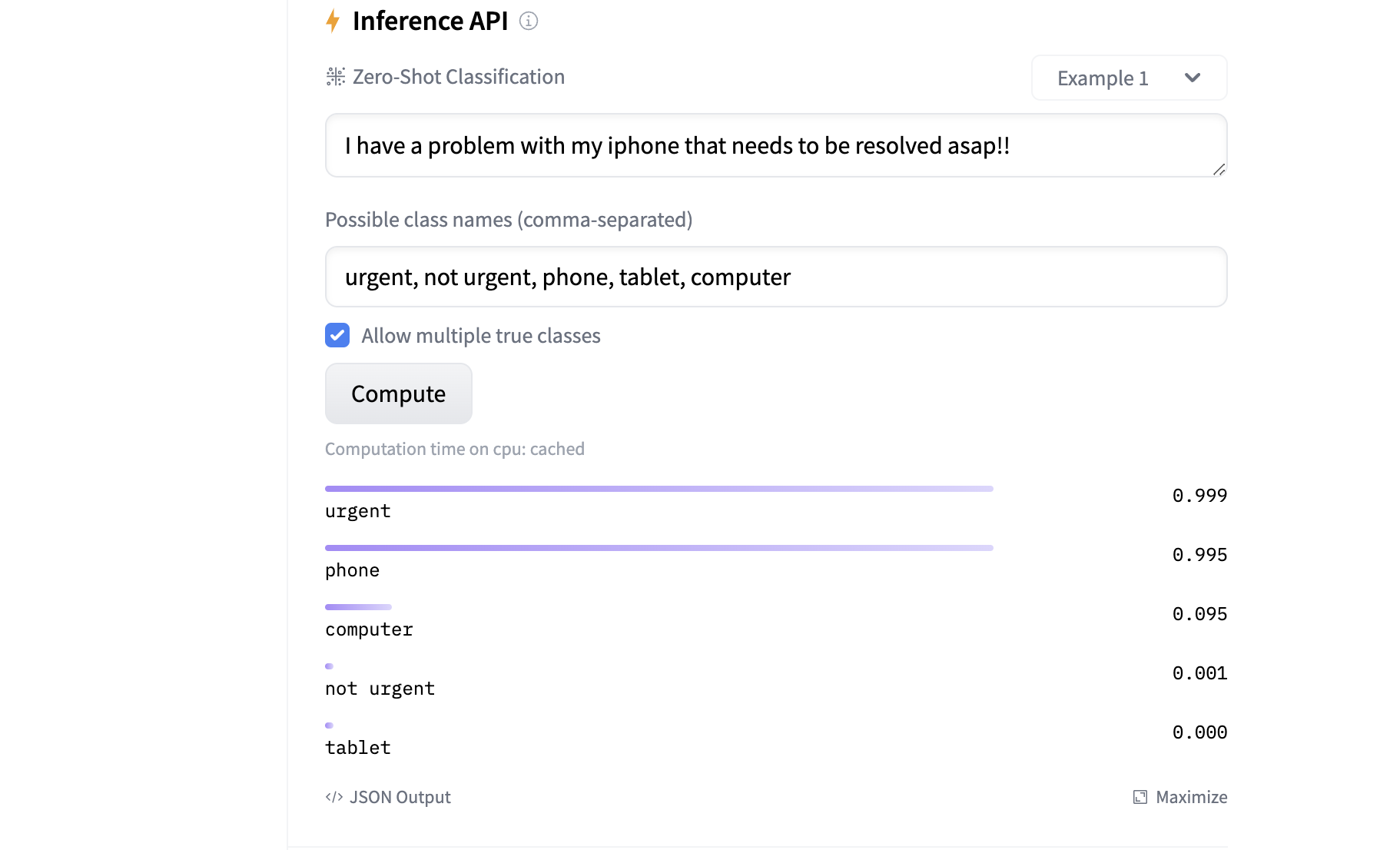
You pass a block of text along with the class names you want to categorize the text into. You then click Compute, and the facebook/bart-large-mnli model assigns a score between 0 and 1 to each class. The numbers represent how likely the model thinks the text belongs to the corresponding class. In this example, the model assigns high scores to the classes urgent and phone. This makes sense because the input text describes an urgent phone issue.

To determine whether a model card is appropriate for your use case, you can review the information within the model card, including the metadata and Inference API features. These are great resources to help you familiarize yourself with the model and determine it’s suitability. And with that primer on Hugging Face and model cards, you’re ready to start running these models in Transformers.

Installing Transformers

Transformers is available on PyPI and you can install it with pip. Open a terminal or command prompt, create a new virtual environment, and then run the following command:

(venv) $ python -m pip install transformers

This command will install the latest version of Transformers from PyPI onto your machine. You’ll also leverage PyTorch to interact with models at a lower level.

You can install PyTorch with the following command:

(venv) $ python -m pip install torch

To verify that the installations were successful, start a Python REPL and import transformers and torch:

>>> import transformers
>>> import torch

If the imports run without errors, then you’ve successfully installed the dependencies needed for this tutorial, and you’re ready to get started with pipelines!

Running Pipelines

Pipelines are the simplest way to use models out of the box in Transformers. In particular, the pipeline() function offers you a high-level abstraction over models in the Hugging Face Model Hub.

To see how this works, suppose you want to use a sentiment classification model. Sentiment classification models take in text as input and output a score that indicates the likelihood that the text has negative, neutral, or positive sentiment. One popular sentiment classification model available in the hub is the cardiffnlp/twitter-roberta-base-sentiment-latest model.

You can run this model with the following code:

>>> from transformers import pipeline

>>> model_name = "cardiffnlp/twitter-roberta-base-sentiment-latest"
>>> sentiment_classifier = pipeline(model=model_name)

>>> text_input = "I'm really excited about using Hugging Face to run AI models!"
>>> sentiment_classifier(text_input)
[{'label': 'positive', 'score': 0.9870720505714417}]

>>> text_input = "I'm having a horrible day today."
>>> sentiment_classifier(text_input)
[{'label': 'negative', 'score': 0.9429882764816284}]

>>> text_input = "Most of the Earth is covered in water."
>>> sentiment_classifier(text_input)
[{'label': 'neutral', 'score': 0.7670556306838989}]

In this block, you import pipeline() and load the cardiffnlp/twitter-roberta-base-sentiment-latest model by specifying the model parameter in pipeline(). When you do this, pipeline() returns a callable object, stored as sentiment_classifier, that you can use to classify text. Once created, sentiment_classifier() accepts text as input, and it outputs a sentiment label and score that indicates how likely the text belongs to the label.

The model scores range from 0 to 1. In the first example, sentiment_classifier predicts that the text has positive sentiment with high confidence. In the second and third examples, sentiment_classifier predicts the texts are negative and neutral, respectively.

If you want to classify multiple texts in one function call, you can pass a list into sentiment_classifier:

>>> text_inputs = [
...     "What a great time to be alive!",
...     "How are you doing today?",
...     "I'm in a horrible mood.",
... ]

>>> sentiment_classifier(text_inputs)
[
    {'label': 'positive', 'score': 0.98383939},
    {'label': 'neutral', 'score': 0.709688067},
    {'label': 'negative', 'score': 0.92381644}
]

Here, you create a list of texts called text_inputs and pass it into sentiment_classifier(). The model wrapped by sentiment_classifier() returns a label and score for each line of text in the order specified by text_inputs. You can see that the model has done a nice job of classifying the sentiment for each line of text!

While every model in the hub has a slightly different interface, pipeline() is flexible enough to handle all of them. For example, a step up in complexity from sentiment classification is zero-shot text classification. Instead of classifying text as positive, neutral, or negative, zero-shot text classification models can classify text into arbitrary categories.

Here’s how you could instantiate a zero-shot text classifier with pipeline():

>>> model_name = "MoritzLaurer/deberta-v3-large-zeroshot-v2.0"
>>> zs_text_classifier = pipeline(model=model_name)

>>> candidate_labels = [
...      "Billing Issues",
...      "Technical Support",
...      "Account Information",
...      "General Inquiry",
... ]

>>> hypothesis_template = "This text is about {}"

In this example, you first load the MoritzLaurer/deberta-v3-large-zeroshot-v2.0 zero-shot text classification model into an object called zs_text_classifier. You then define candidate_labels and hypothesis_template, which are required for zs_text_classifier to make predictions.

The values in candidate_labels tell the model which categories the text can be classified into, and hypothesis_template tells the model how to compare the candidate labels to the text input. In this case, hypothesis_template tells the model that it should try to figure out which of the candidate labels the input text is most likely about.

You can use zs_text_classifier like this:

>>> customer_text = "My account was charged twice for a single order."
>>> zs_text_classifier(
...     customer_text,
...     candidate_labels,
...     hypothesis_template=hypothesis_template,
...     multi_label=True
... )

{'sequence': 'My account was charged twice for a single order.',
 'labels': ['Billing Issues',
            'General Inquiry',
            'Account Information',
            'Technical Support'],
 'scores': [0.98844587,
            0.01255007,
            0.00804191,
            0.00021988]}

Here, you define customer_text and pass it into zs_text_classifier along with candidate_labels and hypothesis_template. By setting multi_label to True, you allow the model to classify the text into multiple categories instead of just one. This means each label can receive a score between 0 and 1 that’s independent of the other labels. When multi_label is False, the model scores sum to 1, which means the text can only belong to one label.

In this example, the model assigned a score of about 0.98 to Billing Issues, 0.0125 to General Inquiry, 0.008 to Account Information, and 0.0002 to Technical Support. From this, you can see that the model believes customer_text is most likely about Billing Issues, and this checks out!

To further demonstrate the power of pipelines, you’ll use pipeline() to classify an image. Image classification is a sub-task of computer vision where a model predicts the likelihood that an image belongs to a specified class. Similar to NLP, image classifiers in the Model Hub can be pretrained on a specific set of labels or they can be trained for zero-shot classification.

In order to use image classifiers from Transformers, you must install Python’s image processing library, Pillow:

(venv) $ python -m pip install Pillow

After installing Pillow, you should be able to instantiate the default image classification model like this:

>>> image_classifier = pipeline(task="image-classification")
No model was supplied, defaulted to google/vit-base-patch16-224
and revision 5dca96d (https://huggingface.co/google/vit-base-patch16-224).

Notice here that you don’t pass the model argument into pipeline(). Instead, you specify the task as image-classification, and pipeline() returns the google/vit-base-patch16-224 model by default. This model is pretrained on a fixed set of labels, so you can specify the labels as you do with zero-shot classification.

Now, suppose you want to use image_classifier to classify the following image of llamas, which you can download from the materials for this tutorial:

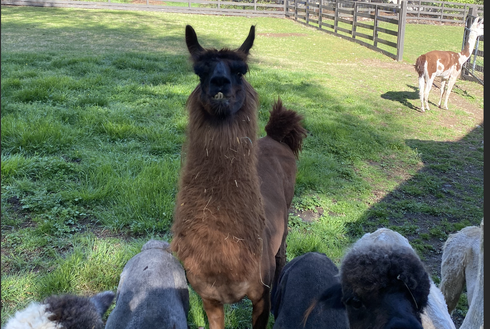
There are a few ways to pass images into image_classifier, but the most straightforward approach is to pass the image path into the pipeline. Ensure the image llamas.png is in the same directory as your Python process, and run the following:

>>> predictions = image_classifier(["llamas.png"])
>>> len(predictions[0])
5

>>> predictions[0][0]
{'label': 'llama',
 'score': 0.9991388320922852}

>>> predictions[0][1]
{'label': 'Arabian camel, dromedary, Camelus dromedarius',
 'score': 8.780974167166278e-05}

>>> predictions[0][2]
{'label': 'standard poodle',
 'score': 2.815701736835763e-05}

Here, you pass the path llamas.png into image_classifier and store the results as predictions. The model returns the five most likely labels. You then look at the first class prediction, predictions[0][0], which is the class the model thinks the image most likely belongs to. The model predicts that the image should be labeled as llama with a score of about 0.99.

The next two most likely labels are Arabian camel and standard poodle, but the scores for these labels are very low. It’s pretty amazing how confident the model is at predicting llama on an image it has never seen before!

The most important takeaway is how straightforward it is to use models out of the box with pipeline(). All you do is pass raw inputs like text or images into pipelines, along with the minimum amount of additional input the model needs to run, such as the hypothesis template or candidate labels. The pipeline handles the rest for you.

While pipelines are great for getting started with models, you might find yourself needing more control over the internal details of a model. In the next section, you’ll learn how to break out pipelines into their individual components with auto classes.

Looking Under the Hood With Auto Classes

As you’ve seen so far, pipelines make it easy to use models out of the box. However, you may want to further customize models through techniques like fine-tuning. Fine-tuning is a technique that adapts a pretrained model to a specific task with potentially different but related data. For example, you could take an existing image classifier in the Model Hub and further train it to classify images that are proprietary to your company.

For customization tasks like fine-tuning, Transformers allows you to access the lower-level components that make up pipelines via auto classes. This section won’t go over fine-tuning or other customizations specifically, but you’ll get a deeper understanding of how pipelines work under the hood by looking at their auto classes.

Suppose you want more granular access and understanding of the cardiffnlp/twitter-roberta-base-sentiment-latest sentiment classifier pipeline you saw in the previous section. The first component of this pipeline, and almost every NLP pipeline, is the tokenizer.

Tokens can be words, subwords, or even characters, depending on the design of the tokenizer. A tokenizer is a component that processes input text and converts it into a format that the model can understand. It does this by breaking the text into tokens and associating those tokens with an ID.

You can access tokenizers using the AutoTokenizer class. To see how this works, take a look at this example:

>>> from transformers import AutoTokenizer

>>> model_name = "cardiffnlp/twitter-roberta-base-sentiment-latest"
>>> tokenizer = AutoTokenizer.from_pretrained(model_name)

>>> input_text = "I really want to go to an island. Do you want to go?"
>>> encoded_input = tokenizer(input_text)
>>> encoded_input["input_ids"]
[0, 100, 269, 236, 7, 213, 7, 41, 2946, 4, 1832, 47, 236, 7, 213, 116, 2]

In this block, you first import the AutoTokenizer class from Transformers. You then instantiate and store the tokenizer for the cardiffnlp/twitter-roberta-base-sentiment-latest model using the .from_pretrained() class method. Lastly, you pass some input_text into the tokenizer and look at the IDs it associates with each token.

Each integer in input_ids is the ID of a token within the tokenizer’s vocabulary. For example, you can already tell that ID 7 corresponds to the token to because it’s repeated multiple times. This might seem a bit cryptic at first, but we can better understand this by using .convert_ids_to_tokens() to convert the IDs back to tokens:

>>> tokenizer.convert_ids_to_tokens(7)
'Ġto'

>>> tokenizer.convert_ids_to_tokens(2946)
'Ġisland'

>>> tokenizer.convert_ids_to_tokens(encoded_input["input_ids"])
['<s>','I','Ġreally','Ġwant','Ġto','Ġgo','Ġto','Ġan','Ġisland','.',
 'ĠDo', 'Ġyou', 'Ġwant', 'Ġto', 'Ġgo', '?', '</s>']

With .convert_ids_to_tokens(), we see that ID 7 and ID 2946 convert to tokens to and island, respectively. The Ġ prefix is a special symbol used to denote the beginning of a new word in contexts where whitespace is used as a separator. By passing encoded_input["input_ids"] into .convert_ids_to_tokens(), you recover the original text input with the additional tokens <s> and </s>, which denote the beginning and end of the text.

You can see how many tokens are in the tokenizer’s vocabulary by looking at the vocab_size attribute:

>>> tokenizer.vocab_size
50265

This particular tokenizer has 50,265 tokens. If you wanted to fine-tune this model, and there were new tokens in your training data, you’d have to add them to the tokenizer with .add_tokens():

>>> new_tokens = [
...     "whaleshark",
...     "unicorn",
... ]

>>> tokenizer.convert_tokens_to_ids(new_tokens)
[3, 3]

>>> tokenizer.convert_ids_to_tokens(3)
'<unk>'

>>> tokenizer.add_tokens(new_tokens)
2

>>> tokenizer.convert_tokens_to_ids(new_tokens)
[50265, 50266]

You first define a list called new_tokens, which has two tokens that aren’t in the tokenizer’s vocabulary by default. When you call .convert_tokens_to_ids(), both of the new tokens map to ID 3. Token ID 3 corresponds to <unk>, which is the default token for input tokens that aren’t in the vocabulary. When you pass new_tokens into .add_tokens(), the tokens are added to the vocabulary and assigned new IDs of 50265 and 50266.

You can also use auto classes to access the model object. For the cardiffnlp/twitter-roberta-base-sentiment-latest model, you can load the model object directly using AutoModelForSequenceClassification:

>>> import torch
>>> from transformers import (
...     AutoTokenizer,
...     AutoModelForSequenceClassification
... )
>>> 
>>> model_name = "cardiffnlp/twitter-roberta-base-sentiment-latest"
>>> 
>>> tokenizer = AutoTokenizer.from_pretrained(model_name)
>>> model = AutoModelForSequenceClassification.from_pretrained(model_name)
>>> model
RobertaForSequenceClassification(
  (roberta): RobertaModel(
    (embeddings): RobertaEmbeddings(
      (word_embeddings): Embedding(50265, 768, padding_idx=1)
      (position_embeddings): Embedding(514, 768, padding_idx=1)
      (token_type_embeddings): Embedding(1, 768)
      (LayerNorm): LayerNorm((768,), eps=1e-05, elementwise_affine=True)
      (dropout): Dropout(p=0.1, inplace=False)
    )
    (encoder): RobertaEncoder(
      (layer): ModuleList(
        (0-11): 12 x RobertaLayer(
          (attention): RobertaAttention(
            (self): RobertaSelfAttention(
              (query): Linear(in_features=768, out_features=768, bias=True)
              (key): Linear(in_features=768, out_features=768, bias=True)
              (value): Linear(in_features=768, out_features=768, bias=True)
              (dropout): Dropout(p=0.1, inplace=False)
            )
            (output): RobertaSelfOutput(
              (dense): Linear(in_features=768, out_features=768, bias=True)
              (LayerNorm): LayerNorm((768,), eps=1e-05, elementwise_affine=True)
              (dropout): Dropout(p=0.1, inplace=False)
            )
          )
          (intermediate): RobertaIntermediate(
            (dense): Linear(in_features=768, out_features=3072, bias=True)
            (intermediate_act_fn): GELUActivation()
          )
          (output): RobertaOutput(
            (dense): Linear(in_features=3072, out_features=768, bias=True)
            (LayerNorm): LayerNorm((768,), eps=1e-05, elementwise_affine=True)
            (dropout): Dropout(p=0.1, inplace=False)
          )
        )
      )
    )
  )
  (classifier): RobertaClassificationHead(
    (dense): Linear(in_features=768, out_features=768, bias=True)
    (dropout): Dropout(p=0.1, inplace=False)
    (out_proj): Linear(in_features=768, out_features=3, bias=True)
  )
)

Here, you add AutoModelForSequenceClassification to your imports and instantiate the model object for cardiffnlp/twitter-roberta-base-sentiment-latest using .from_pretrained(). When you call model in the console, you can see the full string representation of the model. The Roberta model consists of a series of layers that you can access and modify directly.

As an example, take a look at the embeddings layer:

>>> model.roberta.embeddings
RobertaEmbeddings(
  (word_embeddings): Embedding(50265, 768, padding_idx=1)
  (position_embeddings): Embedding(514, 768, padding_idx=1)
  (token_type_embeddings): Embedding(1, 768)
  (LayerNorm): LayerNorm((768,), eps=1e-05, elementwise_affine=True)
  (dropout): Dropout(p=0.1, inplace=False)
)

It’s out of the scope of this tutorial to look at all of the intricacies of the Roberta model, but pay close attention to the word_embeddings layer here. You may have noticed that the first input to Embedding() in the word_embeddings layer is 50265—the exact size of the tokenizer’s vocabulary.

This is because the first embedding layer maps each token in the vocabulary to a PyTorch tensor of size 768. In other words, Embedding(50265, 768) maps all 50,265 tokens in the vocabulary to a PyTorch tensor with 768 elements. To get a better understanding of how this works, you can convert input text to embeddings directly using the embeddings layer:

>>> text = "I love using the Transformers library!"
>>> encoded_input = tokenizer(text, return_tensors="pt")

>>> embedding_tensor = model.roberta.embeddings(encoded_input["input_ids"])
>>> embedding_tensor.shape
torch.Size([1, 9, 768])

>>> embedding_tensor
tensor([[[ 0.0633, -0.0212,  0.0193,  ..., -0.0826, -0.0200, -0.0056],
         [ 0.1453,  0.3706, -0.0322,  ...,  0.0359, -0.0750,  0.0376],
         [ 0.2900, -0.0814,  0.0955,  ...,  0.3262, -0.0559,  0.0819],
         ...,
         [ 0.1059, -0.5638, -0.2397,  ..., -0.2077, -0.0784, -0.0951],
         [ 0.1675, -0.3334,  0.0130,  ..., -0.4127,  0.0121,  0.0215],
         [ 0.1316, -0.0281, -0.0168,  ...,  0.1175,  0.0908, -0.0614]]],
       grad_fn=<NativeLayerNormBackward0>)

In this block, you define text and convert each token to its corresponding ID using tokenizer(). You then pass the token IDs into Roberta’s embeddings layer and store the results as embedding_tensor. Notice how the size of embedding_tensor is [1, 9, 768]. This is because you passed one text input into the embedding layer that had nine tokens in it, and each token was converted to a tensor with 768 elements.

When you look at the embedding_tensor string representation, the first row is the embedding for the <s> token, the second row is for the I token, the third for the love token, and so on. If you wanted to fine-tune the Roberta model with new tokens, you’d first add the new tokens to the tokenizer as you did previously, and then you’d have to update and train the embeddings layer with a 768-element tensor for each new token.

In the full model, the embedding tensor is passed through multiple layers where it’s reshaped, manipulated, and eventually converted to a predicted score for each sentiment class.

You can piece together these auto classes to create the entire pipeline:

>>> import torch
>>> from transformers import (
...     AutoTokenizer,
...     AutoModelForSequenceClassification,
...     AutoConfig
... )

>>> model_name = "cardiffnlp/twitter-roberta-base-sentiment-latest"

>>> config = AutoConfig.from_pretrained(model_name)
>>> tokenizer = AutoTokenizer.from_pretrained(model_name)
>>> model = AutoModelForSequenceClassification.from_pretrained(model_name)

>>> text = "I love using the Transformers library!"
>>> encoded_input = tokenizer(text, return_tensors="pt")

>>> with torch.no_grad():
...     output = model(**encoded_input)
...
>>> scores = output.logits[0]
>>> probabilities = torch.softmax(scores, dim=0)

>>> for i, probability in enumerate(probabilities):
...     label = config.id2label[i]
...     print(f"{i+1}) {label}: {probability}")
...
1) negative: 0.0026470276061445475
2) neutral: 0.010737836360931396
3) positive: 0.9866151213645935

Here, you first import torch along with the auto classes you saw previously. Additionally, you import AutoConfig, which has configuration and metadata for the model. You then store the pipeline name in model_name and instantiate the configuration object, tokenizer, and model object.

Next, you define text and tokenize it with tokenizer(). You then pass the tokenized input, encoded_input, to the model object and store the results as output. You use the torch.no_grad() context manager to speed up model inference by disabling gradient calculations.

After that, you convert the raw model output to scores and then transform the scores to sum to 1 using torch.softmax(). Lastly, you loop through each element in probabilities and output the value along with the associated label, which comes from config.id2label. The results tell you that the model assigns a predicted probability of about 0.9866 to the positive class for the input text.

You can verify that this code gives the same results as the cardiffnlp/twitter-roberta-base-sentiment-latest pipeline you used in the earlier example:

>>> from transformers import pipeline

>>> model_name = "cardiffnlp/twitter-roberta-base-sentiment-latest"
>>> text = "I love using the Transformers library!"

>>> full_pipeline = pipeline(model=model_name)
>>> full_pipeline(text)
[{'label': 'positive', 'score': 0.9866151213645935}]

In this block, you run the same text through the full pipeline and get the exact same predicted score for the positive label.

You now understand how pipelines work under the hood and how you can access and manipulate pipeline components with auto classes. This gives you the tools to create custom pipelines through techniques like fine-tuning, and a deeper understanding of the underlying model.

In the next section, you’ll shift gears and learn how to improve pipeline performance by leveraging GPUs.

Setting Up a Google Colab Notebook

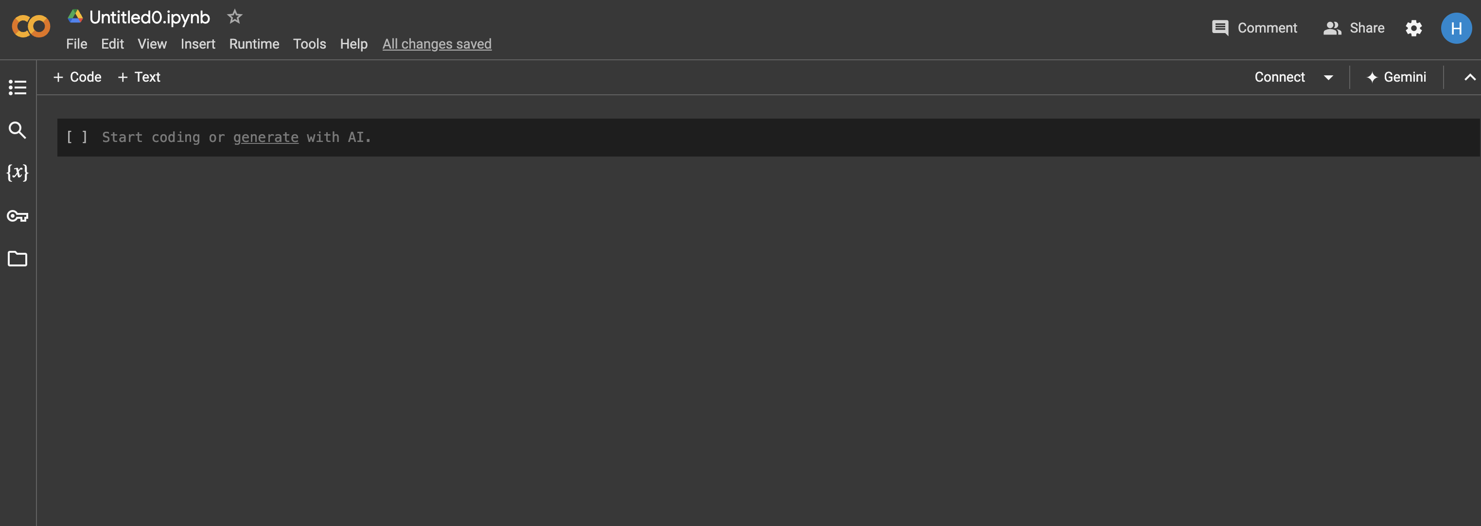
You might not have access to a GPU on your local machine, so in this section, you’ll use Google Colab, a Python notebook interface offered by Google for running pipelines on GPUs for free! To get started, sign into Google Colab and create a new notebook. Once created, your notebook should look something like this:

Next, click the dropdown next to the Connect button and click Change runtime type:

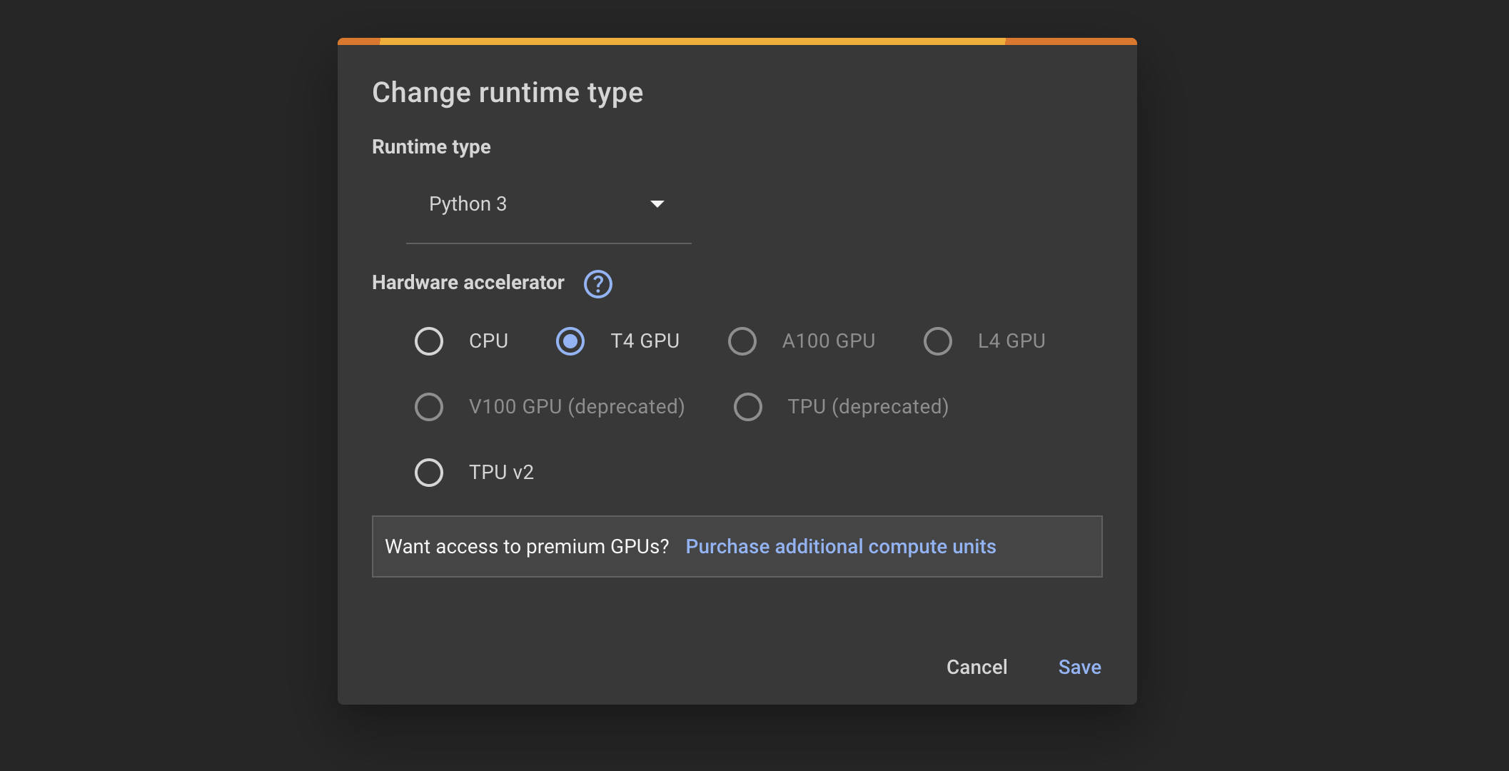
Select the GPU available to you, and click Save. This will connect your notebook to a machine in the cloud with a GPU. Note that if you’re using the free version of Google Colab, GPU availability can vary. This means that if Google Colab receives a high volume of users requesting GPU access, you might have to wait to get access.

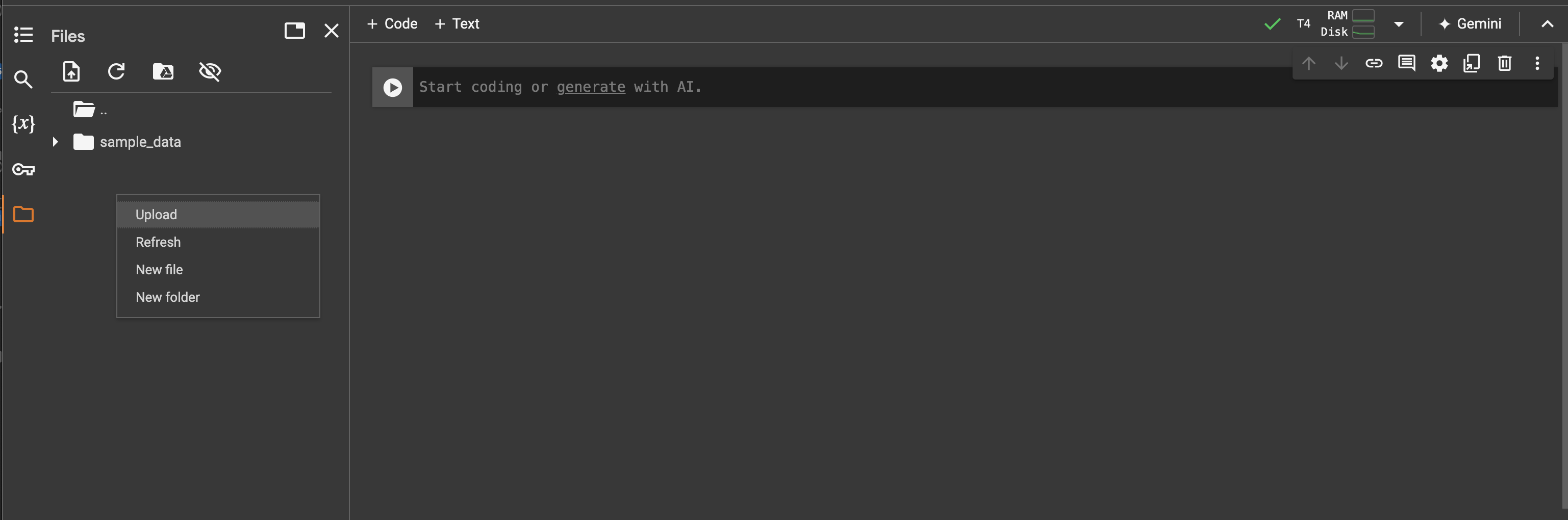
Next, you’ll need to upload the requirements.txt and Scraped_Car_Review_dodge.csv files from this tutorial’s materials to your notebook session. To do this, right-click under the folder tab and choose Upload:

Once uploaded, you should see the two files under the folder tab:

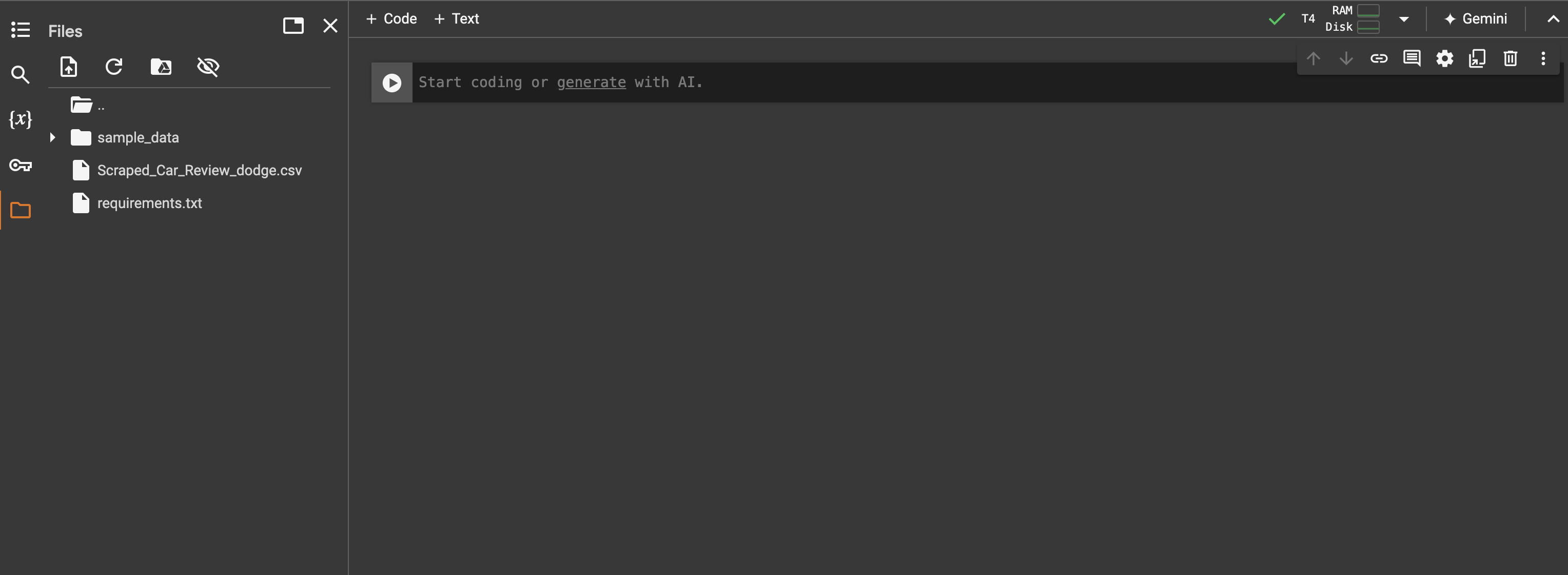
Keep in mind that these files are temporary, and they’ll be deleted whenever your notebook session terminates. If you want to persist files, you can upload them to your Google Drive account and mount it to your notebook.

Lastly, you need to install the libraries specified in the requirements.txt file. You can do this directly from a notebook cell:

In [1]: !pip install -r /content/requirements.txt

Press Shift+Enter, and your requirements should install. Although Google Colab caches popular packages to speed up subsequent installations, you may need to wait a few moments for the installation to finish. Once that completes, you’re ready to start running pipelines on the GPU!

Running Pipelines on GPUs

Now that you have a running notebook with access to a GPU, Transformers makes it easy for you to run pipelines on the GPU. In this section, you’ll run car reviews from the Scraped_Car_Review_dodge.csv file through a sentiment classification pipeline on both the CPU and GPU, and you’ll see how much faster the pipeline runs on the GPU. If you’re interested, you can read more about the car reviews dataset on Kaggle.

To start, define the path to the data and import your dependencies in a new cell:

In [2]: DATA_PATH = "/content/Scraped_Car_Review_dodge.csv"
   ...:
   ...: import time
   ...: from tqdm import tqdm
   ...: import polars as pl
   ...: import torch
   ...: from transformers import (
   ...:     pipeline,
   ...:     TextClassificationPipeline,
   ...: )

Don’t worry if you’re not familiar with some of these dependencies—you’ll see how they’re used in a moment. Next, you can use the Polars library to read in the car reviews and store them in a list:

In [3]: reviews_list = pl.read_csv(DATA_PATH)["Review"].to_list()
   ...: len(reviews_list)
Out[3]: 8499

Here, you read in the Review column from Scraped_Car_Review_dodge.csv and store it in reviews_list. You then look at the length of reviews_list and see there are 8,499 reviews. Here’s what the first review says:

In [4]: reviews_list[0]
Out[4]: " It's been a great delivery vehicle for my 
cafe business good power, economy match easily taken 
care of. Havent repaired anything or replaced anything 
but tires and normal maintenance items. Upgraded tires 
to Michelin LX series helped fuel economy. Would buy 
another in a second"

You’re going to use the cardiffnlp/twitter-roberta-base-sentiment-latest sentiment classifier to predict the sentiment of these reviews using both a CPU and GPU, and you’ll time how long it takes for both. To help you with these experiments, define the following helper function:

In [5]: def time_text_classifier(
   ...:     text_pipeline: TextClassificationPipeline,
   ...:     texts: list[str],
   ...:     batch_size: int = 1,
   ...: ) -> None:
   ...:     """Time how long it takes a TextClassificationPipeline
   ...:        to run inference on a list of texts"""
   ...: 
   ...:     texts_generator = (t for t in texts)
   ...:     pipeline_iterable = tqdm(
   ...:         text_pipeline(
   ...:             texts_generator,
   ...:             batch_size=batch_size,
   ...:             truncation=True,
   ...:             max_length=500,
   ...:         ),
   ...:         total=len(texts),
   ...:     )
   ...: 
   ...:     for result in pipeline_iterable:
   ...:         pass
   ...:

The goal of time_text_classifier() is to evaluate how long it takes a TextClassificationPipeline to make predictions on a list of texts. It first converts the texts to a generator called text_generator, and passes the generator to the text classification pipeline. This turns the pipeline into an iterable that can be looped over to get predictions. The batch_size determines how many predictions the model makes in one pass.

You wrap the text classification pipeline iterator with tqdm() to see your pipeline’s progress as it makes predictions. Lastly, you iterate over pipeline_iterable and use the pass statement since you’re only interested in how long it takes to run. After all predictions are made, tqdm() displays the total runtime.

Next, you’ll instantiate two pipelines, one that runs on the CPU and the other on the GPU:

In [6]: model_name = "cardiffnlp/twitter-roberta-base-sentiment-latest"
   ...: sentiment_pipeline_cpu = pipeline(model=model_name, device=-1)
   ...: sentiment_pipeline_gpu = pipeline(model=model_name, device=0)

Transformers makes it easy for you to specify what hardware your pipeline runs on with the device argument. When you pass an integer to the device argument, you’re telling the pipeline which GPU it should run on. When device is -1, the pipeline runs on the CPU, and any non-negative device number tells the pipeline which GPU to use based on its ordinal rank.

In this case, you likely only have one GPU, so setting device=0 tells the pipeline to run on the first and only GPU. If you had a second GPU, you could set device=1, and so on. You’re now ready to time these two pipelines starting with the CPU:

In [7]: time_text_classifier(sentiment_pipeline_cpu, reviews_list[0:1000])
Out[7]: 100%|██████████| 1000/1000 [05:49<00:00,  2.86it/s]

Here, you time how long it takes sentiment_pipeline_cpu to make predictions on the first 1000 reviews. The results show it took about 5 minutes and 49 seconds. This means sentiment_pipeline_cpu made roughly 2.86 predictions per second.

Now you can run the same experiment for sentiment_pipeline_gpu:

In [8]: time_text_classifier(sentiment_pipeline_gpu, reviews_list[0:1000])
Out[8]: 100%|██████████| 1000/1000 [00:16<00:00, 60.06it/s]

Woah! On the exact same 1000 reviews, sentiment_pipeline_gpu took about 16 seconds to make all the predictions! That’s nearly 61 predictions per second and roughly 21 times faster than sentiment_pipeline_cpu. Keep in mind that the exact run times will vary, but you can run this experiment multiple times to gauge the average time.

You can further optimize the pipeline’s performance by experimenting with batch_size, which is a parameter that determines how many inputs the model processes at one time. For example, if the batch_size is 4, then the model will make predictions of four inputs simultaneously. Check out the performance of cardiffnlp/twitter-roberta-base-sentiment-latest on different batch sizes:

In [9]: batch_sizes = [1, 2, 4, 8, 10, 12, 15, 20, 50, 100]
   ...: for batch_size in batch_sizes:
   ...:     print(f"Batch size: {batch_size}")
   ...:     time_text_classifier(
   ...:         sentiment_pipeline_gpu,
   ...:         reviews_list,
   ...:         batch_size=batch_size
   ...:     )
   ...:
Out[9]:
Batch size: 1
100%|██████████| 8499/8499 [01:50<00:00, 77.02it/s]
Batch size: 2
100%|██████████| 8499/8499 [01:33<00:00, 91.19it/s]
Batch size: 4
100%|██████████| 8499/8499 [01:39<00:00, 85.84it/s]
Batch size: 8
100%|██████████| 8499/8499 [01:47<00:00, 78.76it/s]
Batch size: 10
100%|██████████| 8499/8499 [01:51<00:00, 75.99it/s]
Batch size: 12
100%|██████████| 8499/8499 [01:56<00:00, 73.19it/s]
Batch size: 15
100%|██████████| 8499/8499 [02:01<00:00, 70.16it/s]
Batch size: 20
100%|██████████| 8499/8499 [02:04<00:00, 68.32it/s]
Batch size: 50
100%|██████████| 8499/8499 [02:37<00:00, 53.91it/s]
Batch size: 100
100%|██████████| 8499/8499 [03:08<00:00, 45.15it/s]

Here, you iterate over a list of batch sizes and see how long it takes the pipeline to run through all 8,499 reviews on the corresponding batch size. From the tqdm output, you can see a batch size of 2 resulted in the best performance at about 91 predictions per second.

In general, deciding on an optimal batch size for inference requires experimentation. You should run experiments like this multiple times on different datasets to see which batch size is best on average.

You now know how to run and evaluate pipelines on GPUs! Keep in mind that while most models available in Transformers run best on GPUs, it’s not always feasible to do so. In practice, GPUs can be expensive and resource-intensive, so you have to decide whether the performance gain is necessary and worth the cost for your application. Always experiment and make sure you have a solid understanding of the hardware you want to use.