Random numbers are a very useful feature in many different types of programs, from mathematics and data analysis through to computer games and encryption applications. You may be surprised to learn that it’s actually quite difficult to get a computer to generate true randomness. However, if you’re careful, the NumPy random number generator can generate random enough numbers for everyday purposes.
Maybe you’ve already worked with randomly generated data in Python. While modules like random are great options for producing random scalars, using the numpy.random module will unlock even more possibilities for you.
In this tutorial, you’ll learn how to:
- Generate NumPy arrays of random numbers
- Randomize NumPy arrays
- Randomly select parts of NumPy arrays
- Take random samples from statistical distributions
Before starting this tutorial, you should understand the basics of NumPy arrays. With that knowledge, you’re ready to dive in.
Free Bonus: Click here to download the sample code that shows you how to get random numbers with NumPy.
Understanding the NumPy Pseudo-Random Number Generator
When you ask a computer to perform any task for you, it does so by following a set of instructions defined by an algorithm. When you need it to generate random numbers, the computer uses a pseudo-random number generator (PRNG) algorithm. There are several of these available, some of which are better than others.
To generate random numbers, Python uses the random module, which generates numbers using the Mersenne twister algorithm. While this is still widely used in Python code, it’s possible to predict the numbers that it generates, and it requires significant computing power.
Since version 1.17, NumPy uses the more efficient permuted congruential generator-64 (PCG64) algorithm. This produces less-predictable numbers, as shown by its performance in the industry-standard TestU01 statistical test. PCG64 is also faster and requires fewer resources to work.
Note: While the PCG64 algorithm is certainly an improvement on the Mersenne twister algorithm, it still has some statistical weaknesses. An updated version, PCG64DXSM, addresses these issues. This will become the default in future NumPy releases. On a practical level, you won’t notice any difference, but if you want to know more, see Upgrading PCG64 with PCG64DXSM in the NumPy documentation.
In most of the examples throughout this tutorial, you’ll use the default PCG64 algorithm, although you’ll also try your hand at using the updated PCG64DXSM algorithm.
If you’re interested in learning more about the different types of PRNG algorithms and how the PCG algorithms compare to others, then you should read PCG, A Family of Better Random Number Generators from the developer of PCG.
PRNGs are called pseudo-random because they’re not random! PRNGs are deterministic, which means they generate sequences of numbers that are reproducible. PRNGs require a seed number to initialize their number generation. PRNGs that use the same seed will generate the same numbers.
PRNGs also have a period property, which is the number of iterations they go through before they start repeating. Because the generated numbers depend on the seed, they’re not truly random but are instead pseudo-random.
Because seeds should be random, you need one random number to generate another. For this purpose, PRNGs use the computer hardware clock’s time as their default seed. This is measured to the nanosecond, so running number generators consecutively results in different seed values and therefore different sequences of random numbers. NumPy uses a hashing technique to ensure that the seed is 128 bits long, even if you only supply a 64-bit integer.
The period does mean that the same numbers could reappear. In practice, this isn’t a concern because the period lengths are huge. The period of PCG64, for example, is about 50 billion times the number of atoms that exist inside of you!
Note: If you want to learn more about how random randomly generated numbers actually are, take a look at the tutorial How Random is Random?
The core of NumPy’s number generation is the BitGenerator class. This class allows you to specify an algorithm and seed. To access the random numbers, the BitGenerator is passed into a separate Generator object. Generators have methods that allow you to access a range of random numbers and perform several randomizing operations. The numpy.random module provides this capability.
You may have noticed that the NumPy.random documentation also contains information about the RandomState class. This is a container class for the slower Mersenne twister PRNG. The more modern Generator class has now superseded RandomState, which you should no longer use in new code. However, RandomState is still around for existing legacy applications.
Before you go any further, be aware that the NumPy PRNGs are not suitable for cryptographic purposes. They’re only suitable for data analysis tasks. If you need random numbers for cryptographic purposes, then you need a cryptographically secure pseudo-random number generator (CSPRNG).
Generating Random Data With the NumPy Random Number Generator
Now that you understand a computer’s capabilities for generating random numbers, in this section, you’ll learn how to generate both floating-point numbers and integers randomly using NumPy. After generating individual numbers, you’ll learn how to generate NumPy arrays of random numbers.
Random Numbers
If you’re happy to let NumPy perform all of your random number generation work for you, you can use its default values. In other words, your BitGenerator will use PCG64 with a seed from the computer’s clock. To facilitate the defaults, NumPy provides a very handy default_rng() function. This sets everything up for you and returns a reference to a Generator object for you to use to produce random numbers using its range of powerful methods.
To begin with, this code generates a floating-point number using NumPy’s defaults:
>>> import numpy as np

>>> default_rng = np.random.default_rng()
>>> default_rng
'Generator(PCG64) at 0x1E9F2ABBF20'

>>> default_rng.random()
0.47418635476614734
As you can see, BitGenerator uses PCG64. To actually generate a pseudo-random number, you call the generator’s .random() method. To satisfy yourself that the code is indeed generating a random number, run it several times and notice that you get a different number each time. Remember, this is because the seed value passed will be different.
By default, Generator.random() returns a 64-bit float in the half-open interval [0.0, 1.0). This notation is used to define a number range. The [ is the closed parameter and indicates inclusivity. In this example, 0.0 could be one of the numbers randomly generated. The ) is the open parameter and indicates the value 1.0 is just beyond what could be generated. In other words, [0.0, 1.0) defines the range 0.0 ≤ x < 1.0.
Note:: If you really need the more powerful PCG64DXSM algorithm, applying it is pretty straightforward:
>>> from numpy.random import Generator, PCG64DXSM
>>> pcg64dxsm_rng = Generator(PCG64DXSM())
>>> pcg64dxsm_rng.random()
0.3472568589560456
You first create a Generator object explicitly, and this time you pass it the PCG64DXSM BitGenerator. When you call the .random() method, you’re again generating a random number, but this time PCG64DXSM guarantees less predictable output than the default PCG64 BitGenerator is capable of producing. Of course, you can’t tell this from looking at a single sample, but have faith in the mathematicians. The above numbers are less predictable.
Earlier you learned how passing a seed value determines the sequence of random numbers generated. Recall that passing identical seed values into separate BitGenerator objects forces them to produce the same output. In the following example, you’ll see this for yourself.
In the code snippet below, you seed two separate identical Generator objects, both with a seed value of 100:
>>> rng1 = np.random.default_rng(seed=100)
>>> rng1.random()
0.7852902058808499
>>> rng1.random()
0.7142492625022044

>>> rng2 = np.random.default_rng(seed=100)
>>> rng2.random()
0.7852902058808499
>>> rng2.random()
0.7142492625022044
As expected, each Generator has generated two numbers, but they’re actually pseudo-random numbers! As you can see, the results give you a feeling of déjà vu. Seeding Generator objects identically always produces identical results! It doesn’t matter if both use the default PCG64 or both use the updated PCG64DXSM. The results would still be identical.
The random() method also includes a dtype parameter, which is rarely used. By default, this is set to np.float64, which generates 64-bit floats. If you set this parameter to np.float32, you can generate 32-bit floats instead.
Random Floating-Point Numbers
You already know the .random() method will happily generate random floating-point numbers in the range [0.0, 1.0). Suppose you want to specify your own range. Unfortunately, this isn’t directly possible with .random(), unless you start adding some arithmetic to its output. To specify a range of floats, you can use the .uniform() method.
As you can probably guess from the .uniform() method’s signature, it defaults to generating a floating-point number in the same way that .random() does. However, unlike with .random(), you can optionally specify your own low and high parameters. The .uniform() method also contains a size parameter. You’ll learn more about this when you learn to generate random NumPy arrays later.
In its most basic form, you can call the .uniform() method with no parameters:
>>> import numpy as np
>>> rng = np.random.default_rng()

>>> rng.uniform()
0.5425301829704396
When you run the above code,.uniform() will generate a single random floating-point number in the range [0, 1). In other words, the lowest number will be 0, while the largest number will be just less than 1. Should you want a number from 0 to just before 10, for example, you’d need to multiply the output by 10. However, this is limited because the lower bound will always be zero, and the coding is unclear.
A far better way is to utilize the real power of .uniform() by passing in its low and high parameters:
>>> rng.uniform(low=3.4, high=5.6)
4.656018709365851
Here, because you set low=3.4 and high=5.6, the .uniform() method generates another single float, but this time in the range [3.4, 5.6). Again, remember, 3.4 is inclusive, while 5.6 is exclusive.
You may wonder why a method used to generate floats is called .uniform(). The .uniform() method draws its numbers randomly from a uniform probability distribution. A uniform probability distribution means each of the values in the specified range [low, high) has an equal chance of being chosen. You’ll see later that this isn’t the only type of probability distribution NumPy supports.
Random Integer Numbers
If you need to, you can also generate random integers. You do this using the Generator object’s .integers() method.
In its most basic form, you use .integers() with its one mandatory parameter:
>>> import numpy as np

>>> rng = np.random.default_rng()
>>> for i in range(5):
...     rng.integers(3)
...
1
2
0
1
2
When you call .integers() with a single parameter, that parameter defines the upper exclusive bound of the numbers generated. In this example, because you’ve passed in 3, the possibe outputs are in the range [0, 3). In other words, you might get 0, 1, or 2.
If you call .integers() five times using a for loop and the range() function, then it produces five values.
While you might find the above example your most common way of using .integers(), the method is actually far more flexible. Unfortunately, it’s also a little confusing. The .integers() method’s signature includes three parameters for defining the range of numbers from which the method will generate your random numbers: low, high, and endpoint. Unfortunately, they aren’t quite as intuitive to use as their names suggest.
The low parameter is the only one that’s mandatory. While its name suggests its value will define the lowest integer that the .integers() function can select, this is actually only true if you provide a value for the high parameter as well. So if you set low=1 and high=4, then the .integers() method will select a random number in the range [1, 4):
>>> for count in range(5):
...     rng.integers(low=1, high=4)
...
3
2
3
1
2
Here, you’ve only generated the numbers 1, 2, and 3. Once again, while low is possible, high isn’t.
Now, here’s where confusion may occur. If you pass only a low argument and accept the default high value of None, then .integers() sets its low parameter to 0 and use the value you provide for the upper limit. So, for example, if you call .integers(low=7) or .integers(7), although 7 is the low parameter, the method will return a value in the range [0, 7):
>>> for count in range(5):
...     rng.integers(low=7)
...
3
4
2
6
0
In the above code, you generate integers in the range from 0 to 6. Naming low here is misleading. Instead you should call rng.integers(7) or use the more explicit rng.integers(low=0, high=7) to do the same thing. In general, you should always include high if you pass low as a keyword argument.
The third parameter that defines the range is the endpoint parameter, which determines whether the interval includes the high value. Remember how the default is a half-open interval? That’s because endpoint defaults to False, meaning the sample interval is [low, high). However, if you set it to True, then the interval becomes inclusive at both ends, [low, high]. Knowing this, you can now write an inclusive interval:
>>> for count in range(5):
...     rng.integers(low=1, high=4, endpoint=True)
...
1
4
4
3
2

>>> for count in range(5):
...     rng.integers(7, endpoint=True)
...
5
7
6
2
0
This time, the first loop will generate either 1, 2, 3, or 4. The second loop will generate numbers in the range 0 to 7, inclusive. Setting endpoint=True might make your integer intervals more intuitive.
The .integers() method produces 64-bit integers by default. This is because its dtype parameter is set to np.int64. If you set dtype to np.int32, then you’d obtain 32-bit integers instead.
Random NumPy Arrays
When working with NumPy, you may wish to produce a NumPy array containing random numbers. You do this using the size parameter of either the .random(), .uniform(), or .integers() method of the Generator object. In all three methods, the default value of size is None, which causes a single number to be generated. However, if you assign a tuple to size, then you’ll generate an array.
In the example below, you generate a variety of NumPy arrays using different-size tuples:
>>> import numpy as np

>>> rng = np.random.default_rng()

>>> rng.random(size=(5,))
array([0.18097689, 0.19402707, 0.82936953, 0.29470017, 0.73697751])

>>> rng.random(size=(5, 3))
array([[0.85815152, 0.44158512, 0.49992378],
       [0.99656444, 0.40376014, 0.93886646],
       [0.31424733, 0.23561498, 0.43465744],
       [0.02478389, 0.60644643, 0.52940267],
       [0.54349223, 0.77175087, 0.2834884 ]])

>>> rng.random(size=(3, 4, 2))
array([[[0.78538958, 0.93149463],
        [0.73405027, 0.32193268],
        [0.14362809, 0.59825765],
        [0.07675847, 0.0434828 ]],

       [[0.28681395, 0.66925531],
        [0.59575724, 0.18366003],
        [0.54722312, 0.02620217],
        [0.06019602, 0.48735061]],

       [[0.40764258, 0.00756601],
        [0.32556725, 0.44165999],
        [0.05679186, 0.01690106],
        [0.87091753, 0.46327738]]])
If you want to create a one-dimensional array, then you set the size parameter to an integer or a tuple with a single element. Either size=x or size=(x, ) allows you to generate a one-dimensional array with x elements.
Similarly, if you want to create a two-dimensional array with x rows and y columns, then you use size=(x, y). Setting the size parameter to a tuple with the elements (x, y, z) allows you to generate a three-dimensional array with x sets of y rows and z columns.
In this next example, you randomly generate two arrays, but this time, you specify the acceptable ranges of numbers:
>>> rng = np.random.default_rng()
>>> rng.integers(size=(2, 3), low=1, high=5)
array([[4, 2, 3],
       [1, 1, 2]], dtype=int64)

>>> rng.uniform(size=(2, 3), low=1, high=5)
array([[4.97441068, 1.02042664, 1.43584549],
       [2.87965746, 1.99063036, 2.86212453]])
As you can see, the first array contains integers, while the second one contains floating-point numbers. Both are in the range [1, 5).
Now that you’ve gained confidence in creating random integers and floats, both individually and in NumPy arrays, you’ll next see how you can randomize NumPy arrays themselves.
Randomizing Existing NumPy Arrays
Once you have a NumPy array, regardless of whether you’ve generated it randomly or obtained it from a more ordered source, there may be times when you need to select elements from it randomly or reorder its structure randomly. You’ll learn how to do this next.
Selecting Array Elements Randomly
Suppose you have a NumPy array of data collected from a survey, and you wish to use a random sample of its elements for analysis. The Generator object’s .choice() method allows you to select random samples from a given array in a variety of different ways. You give this a whirl in the next few examples:
>>> import numpy as np

>>> rng = np.random.default_rng()

>>> input_array_1d = np.array([1, 2, 3, 4, 5, 6, 7, 8, 9, 10, 11, 12])
>>> rng.choice(input_array_1d, size=3, replace=False)
array([ 6, 12, 10])

>>> rng.choice(input_array_1d, size=(2, 3), replace=False)
array([[ 8, 12, 11],
       [10,  7,  5]])
In this example, you’re analyzing a one-dimensional NumPy array. The first .choice() call creates a one-dimensional array containing three elements chosen randomly from the original array. The second .choice() call creates a two-by-three array of six random elements from the original data.
The previous code makes use of the replace parameter. If you set replace to False, then you can’t select the same element more than once. By default, it’s set to True, meaning the same element might be selected multiple times. This is analogous to selecting a ball from a bag, replacing it, and then selecting again. When you need to avoid duplication, you should set replace to False.
One point to note is that the .choice() method selects elements based on their position in the original array. Should the same value appear twice in the original data, you could end up having both values selected regardless of which replace parameter setting you use.
Selecting Rows and Columns Randomly
Suppose you wanted to randomly select one or more entire rows or columns from an array. The .choice() method allows this by means of its axis parameter. The axis parameter allows you to specify the direction in which you wish to analyze. For a two-dimensional array, setting axis=0, which is the default, means that you’ll be analyzing by row, while setting axis=1 means that you’ll analyze by column.
Here are some examples of random selection in both directions:
>>> import numpy as np

>>> rng = np.random.default_rng()

>>> input_array = np.array([[1, 2, 3], [4, 5, 6], [7, 8, 9], [10, 11, 12]])

>>> rng.choice(input_array, size=2)
array([[10, 11, 12],
       [10, 11, 12]])

>>> rng.choice(input_array, size=2, axis=1)
array([[ 2,  1],
       [ 5,  4],
       [ 8,  7],
       [11, 10]])
You’re using an original NumPy array with four rows and three columns. The first analysis will randomly select two unique rows. In this case, the same row has been selected twice, but this won’t always be the case. As you might expect, the output is a two-by-three NumPy array. The second analysis randomly selects two columns. Again, duplicates may occur when you run the code, but you haven’t gotten any on this occasion.
Note: In the examples involving NumPy arrays, you’re limiting the size to a two-dimensional array for the sake of brevity. The same principles apply to higher-dimensional arrays. You simply set axis to 2, 3, or some higher n value.
To prevent the possibility of the same row or column being chosen multiple times, you set the replace parameter of .choice() to False, rather than its default value of True:
>>> rng.choice(input_array, size=3, replace=False)
array([[10, 11, 12],
       [ 1,  2,  3],
       [ 4,  5,  6]])
You can run the above code as many times as you wish, and you’ll never see any row—or column if axis was set to 1—more than once!
The .choice() method also contains a shuffle parameter that adds in an extra layer of randomness. It allows entire rows—or columns if axis=1—to be reordered after their initial random selection. Individual element order will remain the same within each row or column.
For shuffle to have an effect, you must first set replace to False. That effectively makes the shuffling operation available, but only if shuffle is at its default of True. If you set shuffle to False or set replace to True, then the additional shuffling operation doesn’t occur. In the next few examples, you’ll explore the effects of changing replace and shuffle. Pay careful attention to the output data and its order:
>>> rng = np.random.default_rng(seed=100)
>>> rng.choice(input_array, size=3, replace=False, shuffle=False)
array([[4, 5, 6],
       [7, 8, 9],
       [1, 2, 3]])
As the output above shows, you’ve selected three rows from the array. These have been displayed in their selected order. Setting shuffle to False removes the extra shuffle operation that NumPy otherwise does by default, so you’ve sped up your code. Although replace made shuffling a possibility, setting shuffle to False prevented it from occurring.
To add more randomization, you can keep the default by omitting shuffle, or set shuffle to True explicitly:
>>> rng = np.random.default_rng(seed=100)
>>> rng.choice(input_array, size=3, replace=False, shuffle=True)
array([[1, 2, 3],
       [4, 5, 6],
       [7, 8, 9]])
This time, the same three rows were selected because the same seed value was used, but the shuffle parameter has reordered them. By setting shuffle to True, you’ve shuffled the output.
Try running the previous code repeatedly, and you’ll find that the output each time is identical. Not only is the original row selection pseudo-random, but the subsequent shuffling is pseudo-random as well! Both are based on the seed.
Now if you set replace to True, effectively switching shuffle off, then you’re in for a surprise:
>>> rng = np.random.default_rng(seed=100)
>>> rng.choice(input_array, size=3, replace=True, shuffle=False)
array([[10, 11, 12],
       [10, 11, 12],
       [ 1,  2,  3]])

>>> rng = np.random.default_rng(seed=100)
>>> rng.choice(input_array, size=3, replace=True, shuffle=True)
array([[10, 11, 12],
       [10, 11, 12],
       [ 1,  2,  3]])
When you run the code this time, both outputs are identical. This is because both seed values are identical, and shuffle only has an effect if replace is set to False. However, the selected rows are different from those selected in the previous code, despite the fact that the seed values have remained the same.
Remember, the seed value that you explicitly provide to a PRNG is actually only the number it uses to calculate its real seed. In this case, the value of the replace parameter contributes to the calculation.
Shuffling Arrays Randomly
It’s possible for you to randomize the order of the elements in a NumPy array by using the Generator object’s .shuffle() method. Although you can reach for it in several use cases, a very common application is a card game simulation.
To begin with, you create a function that produces a NumPy array of concatenated strings representing the various cards in a deck, albeit without the jokers:
>>> import numpy as np

>>> def create_deck():
...     RANKS = "2 3 4 5 6 7 8 9 10 J Q K A".split()
...     SUITS = "♣ ♢ ♡ ♠".split()
...     return np.array([r + s for s in SUITS for r in RANKS])
...
>>> create_deck()
array(['2♣', '3♣', '4♣', '5♣', '6♣', '7♣', '8♣', '9♣', '10♣', 'J♣', 'Q♣',
       'K♣', 'A♣', '2♢', '3♢', '4♢', '5♢', '6♢', '7♢', ...,
       '7♠', '8♠', '9♠', '10♠', 'J♠', 'Q♠', 'K♠', 'A♠'], dtype='<U3')
The create_deck() function returns a NumPy array containing strings such as "2♣", "3♢", "8♡", and "K♠". As you can see, it does this by defining two constants containing the card ranks and their suits, and then it uses a list comprehension to create a Python list, which is then converted into a NumPy array.
Now suppose you want to draw three cards randomly from the deck after a shuffle. The .shuffle() method allows you to modify an array in place by shuffling its contents. By performing the shuffle in place, you save valuable memory space:
>>> rng = np.random.default_rng()
>>> deck_of_cards = create_deck()

>>> rng.shuffle(deck_of_cards)
>>> deck_of_cards[0:3]
array(['4♡', '6♠', '2♠'], dtype='<U3')

>>> rng.shuffle(deck_of_cards)
>>> deck_of_cards[0:3]
array(['K♠', '2♣', '6♠'], dtype='<U3')
Your code shuffles the Numpy array card deck and then displays the first three elements—that is, the top three cards—from the shuffled version. You then reshuffle the deck and draw the top three cards again. Well done if you noticed that you performed both shuffles on the complete deck!
Although you could’ve used the .choice() method that you learned about earlier to select the cards, the .shuffle() method is a better option because it actually randomizes the array elements in place. This saves memory.
Reordering Arrays Randomly
Previously, you learned how to select entire rows or columns of a NumPy array at random. Now suppose you wanted to randomize the elements of a multidimensional array. The generator offers .shuffle() that you’ve seen already, as well as the .permutation() and .permuted() methods for this purpose.
The .permutation() method randomly rearranges entire rows or columns. In other words, the elements within each row or column will stay in those rows and columns, but their order will be changed.
To illustrate these methods, you’ll use an altered version of your create_deck() function:
>>> import numpy as np

>>> def create_high_cards():
...     HIGH_CARDS = "10 J Q K A".split()
...     SUITS = "♣ ♢ ♡ ♠".split()
...     return np.array([r + s for s in SUITS for r in HIGH_CARDS])
...
This time, you produce a deck containing only the tens, aces, and faces. This will make the results of the next few examples easier for you to see.
The initial deck looks like this:
>>> NUMBER_OF_SUITS = 4
>>> NUMBER_OF_RANKS = 5
>>> high_deck = create_high_cards().reshape((NUMBER_OF_SUITS, NUMBER_OF_RANKS))
>>> high_deck
array([['10♣', 'J♣', 'Q♣', 'K♣', 'A♣'],
       ['10♢', 'J♢', 'Q♢', 'K♢', 'A♢'],
       ['10♡', 'J♡', 'Q♡', 'K♡', 'A♡'],
       ['10♠', 'J♠', 'Q♠', 'K♠', 'A♠']], dtype='<U3')
As you can see, the suit order is ♣, ♢, ♡, and ♠, in ascending order from ten to ace.
Now you want to organize the cards from each suit in a random order. To do this, you randomize the position of the rows within the array:
>>> NUMBER_OF_SUITS = 4
>>> NUMBER_OF_RANKS = 5
>>> high_deck = create_high_cards().reshape((NUMBER_OF_SUITS, NUMBER_OF_RANKS))

>>> rng = np.random.default_rng()
>>> rng.permutation(high_deck, axis=0)
array([['10♡', 'J♡', 'Q♡', 'K♡', 'A♡'],
       ['10♢', 'J♢', 'Q♢', 'K♢', 'A♢'],
       ['10♣', 'J♣', 'Q♣', 'K♣', 'A♣'],
       ['10♠', 'J♠', 'Q♠', 'K♠', 'A♠']], dtype='<U3')

>>> rng.permutation(high_deck, axis=0)
array([['10♢', 'J♢', 'Q♢', 'K♢', 'A♢'],
       ['10♠', 'J♠', 'Q♠', 'K♠', 'A♠'],
       ['10♡', 'J♡', 'Q♡', 'K♡', 'A♡'],
       ['10♣', 'J♣', 'Q♣', 'K♣', 'A♣']], dtype='<U3')
You populate the initial array using your new create_high_deck() function. This time, you reshape the array into four rows of suits and five columns of card ranks. Then the .permutation() method works row-wise because axis=0. It randomizes the position of each row, but the content of each row remains in its original order.
Also note that the original high_deck is untouched. The previous operations randomized copies of the deck:
>>> high_deck
array([['10♣', 'J♣', 'Q♣', 'K♣', 'A♣'],
       ['10♢', 'J♢', 'Q♢', 'K♢', 'A♢'],
       ['10♡', 'J♡', 'Q♡', 'K♡', 'A♡'],
       ['10♠', 'J♠', 'Q♠', 'K♠', 'A♠']], dtype='<U3')
The suits are still in the original order. Now say you want to organize the cards from each value in a random order. To do this, you randomize the position of the columns:
>>> rng.permutation(high_deck, axis=1)
array([['10♣', 'Q♣', 'A♣', 'J♣', 'K♣'],
       ['10♢', 'Q♢', 'A♢', 'J♢', 'K♢'],
       ['10♡', 'Q♡', 'A♡', 'J♡', 'K♡'],
       ['10♠', 'Q♠', 'A♠', 'J♠', 'K♠']], dtype='<U3')

>>> rng.permutation(high_deck, axis=1)
array([['Q♣', 'K♣', 'J♣', 'A♣', '10♣'],
       ['Q♢', 'K♢', 'J♢', 'A♢', '10♢'],
       ['Q♡', 'K♡', 'J♡', 'A♡', '10♡'],
       ['Q♠', 'K♠', 'J♠', 'A♠', '10♠']], dtype='<U3')
In the above code, the .permutation() method works column-wise because axis=1. This time, you’ve randomized the position of each column with .permutation(), but the content of each column remains in the initial order. As you can see, the queens have taken the place of the ten rank as the first column, but you’ll notice that the suits are in the same, original order. That’s because you’ve rearranged the columns but kept the rows intact.
It’s easy to become confused when comparing the output from this new .permutation() method and from your earlier .shuffle() method. Both methods rearrange array elements in the same way. The difference is that the .permutation() method creates a new array of results, while .shuffle() updates the original array.
In the examples that you just coded, the .permutation() method randomized the original array. Each call to .permutation() resulted in a randomized copy of the original array.
With the .shuffle() method, you would’ve replaced the original array with the randomized version.
As before, you start off by creating a deck of high cards:
>>> NUMBER_OF_SUITS = 4
>>> NUMBER_OF_RANKS = 5
>>> high_deck = create_high_cards().reshape((NUMBER_OF_SUITS, NUMBER_OF_RANKS))
As you can see, the four suits of the high cards are in this mini-deck. Pay attention to the order of the cards and the fact that you’re referencing them through a variable named high_cards.
Next you shuffle the cards:
>>> rng = np.random.default_rng()
>>> rng.shuffle(high_deck, axis=0)
>>> high_deck
array([['10♢', 'J♢', 'Q♢', 'K♢', 'A♢'],
       ['10♠', 'J♠', 'Q♠', 'K♠', 'A♠'],
       ['10♡', 'J♡', 'Q♡', 'K♡', 'A♡'],
       ['10♣', 'J♣', 'Q♣', 'K♣', 'A♣']], dtype='<U3')
As you can see, setting the axis parameter to 0 has caused the row-order to be randomized. However, the content of each row remains the same.
Now carefully watch what happens when you call .shuffle() a second time:
>>> rng.shuffle(high_deck, axis=1)
>>> high_deck
array([['J♢', 'A♢', 'K♢', '10♢', 'Q♢'],
       ['J♠', 'A♠', 'K♠', '10♠', 'Q♠'],
       ['J♡', 'A♡', 'K♡', '10♡', 'Q♡'],
       ['J♣', 'A♣', 'K♣', '10♣', 'Q♣']], dtype='<U3')
Again, as expected, because you’ve set axis to 1, the column order is randomized. However, the content of each column remains the same. This is because .shuffle() has randomized the previously randomized card deck. In contrast, .permutation() wouldn’t have done this because it would’ve randomized the original, unrandomized version of the deck.
As a final point, you can make both .permutation() and .shuffle() do the same thing. To do this, you would use high_cards=rng.permutation(high_cards, axis=0) or rng.shuffle(high_cards, axis=0). Do remember, however, that your results will probably be different due to the randomization effects.
The .permuted() method randomizes row or column elements independently of the other rows or columns and places the result into a new array. This is best seen by example.
Suppose you wanted to mix up the rows:
>>> NUMBER_OF_SUITS = 4
>>> NUMBER_OF_RANKS = 5
>>> high_deck = create_high_cards().reshape((NUMBER_OF_SUITS, NUMBER_OF_RANKS))

>>> rng = np.random.default_rng()
>>> rng.permuted(high_deck, axis=0)
array([['10♡', 'J♠', 'Q♠', 'K♠', 'A♠'],
       ['10♢', 'J♣', 'Q♡', 'K♣', 'A♣'],
       ['10♣', 'J♡', 'Q♣', 'K♢', 'A♡'],
       ['10♠', 'J♢', 'Q♢', 'K♡', 'A♢']], dtype='<U3')
The .permuted() method works row-wise (axis=0) on the original array. In other words, it changes the content in each row independently of the other rows. Practically, this means that it randomly rearranges the elements of each column. Each column still contains the same cards, but their order is randomized. As a result, the rows contain different suits. In other words, you’ve randomly shuffled all of the value cards.
As you’ve probably guessed, you could also mix up the columns:
>>> rng.permuted(high_deck, axis=1)
array([['J♣', 'A♣', '10♣', 'Q♣', 'K♣'],
       ['K♢', 'A♢', 'J♢', 'Q♢', '10♢'],
       ['J♡', 'K♡', '10♡', 'Q♡', 'A♡'],
       ['J♠', 'Q♠', 'A♠', '10♠', 'K♠']], dtype='<U3')
This time, you’re working column-wise (axis=1) on the original array. Now you’re changing the content in each column independently of the other columns. Practically, you’re randomly rearranging the elements of each row. Each row still contains the same cards, but their order is randomized. As a result, the columns contain different suits. In other words, you’ve randomly shuffled the same-suit cards.
Finally, suppose you wanted to completely randomize the deck:
>>> rng.permuted(rng.permuted(high_deck, axis=1), axis=0)
array([['A♡', 'Q♡', 'A♢', 'K♡', 'J♡'],
       ['Q♢', 'Q♠', '10♡', 'J♠', 'K♣'],
       ['10♠', 'J♣', 'K♠', 'A♣', 'K♢'],
       ['Q♣', 'J♢', '10♣', '10♢', 'A♠']], dtype='<U3')
To perform a complete shuffle, you call the .permuted() method twice—first row-wise and then column-wise. As a result, you’ve randomized all the elements. This time, you’ve shuffled the entire deck, so it’s ready for dealing. Also note that you could alternatively use rng.permuted(rng.permuted(high_cards, axis=0), axis=1). This would still randomize everything to the same level.
Selecting Random Poisson Samples
The Poisson distribution is a popular probability distribution that you can use to determine the probability that a specific number of events will occur, assuming you know the average number of such events occurring. This is usually measured over a period of time.
As an example of the kinds of problems that the Poisson statistical distribution can help you solve, consider the following. Suppose a school safety department wants to investigate the traffic passing a school. They know, on average, one car passes the school every fifteen seconds. The safety department wants to know the probability of each of the following occurring:
- No cars will pass in any given minute.
- Four cars will pass in any given minute.
- Eight cars will pass in any given minute.
To calculate this, you use the Poisson probability mass function (PMF).
The probability of some random variable, X, taking on some discrete value, k, is given by:

Here, λ is the mean number of events that you expect to occur in the timescale under consideration, e is Euler’s constant (2.72), and k is the number of events whose probability you wish to determine.
Looking back at the cars example, you can assume the answers follow a Poisson distribution. The example asks you to determine the probabilities for zero, four, and eight cars passing over a period of one minute. The first value that you need to determine is λ. You know that one car passes, on average, every fifteen seconds, so the average number of cars passing per minute is four. This means λ equals four.
You then need to use the above formula to work out the probabilities. You can do that with the following code:
>>> import math

>>> lam = 4
>>> cars_per_minute = [0, 4, 8]

>>> for cars in cars_per_minute:
...     probability = lam**cars * math.exp(-lam) / math.factorial(cars)
...     print(f"P({cars}) = {probability:.1%}")
...
'P(0) = 1.8%'
'P(4) = 19.5%'
'P(8) = 3.0%'
You’ve set the lambda parameter, lam, to four and have added the desired set of k values, cars_per_minute, to a list. You’ve passed each element of the list into the formula and printed the results.
The main point that you should take away from his example is the three answers—1.8, 19.5, and 3.0 percent—all follow a Poisson probability distribution.
To allow you to visualize this, you could run the previous calculation again with more values and plot them. One way to do this is to take advantage of NumPy’s vectorization capabilities:
import numpy as np
import matplotlib.pyplot as plt
from scipy.special import factorial

lam = 4
k_values = np.arange(0, 30)
probabilities = np.power(lam, k_values) * np.exp(-lam) / factorial(k_values)

plt.plot(k_values, probabilities, "ro")
plt.title("Sample Poisson Distribution.")
plt.xlabel("k")
plt.ylabel("P(k)")
plt.show()
To create the plot, you must install and import two additional libraries. The matplotlib.pyplot library allows you to create a visualization of the data. The scipy.special library includes a factorial() function that can operate on each element of a NumPy array.
The code once more assumes lambda to be four, but this time, it works out the probability of thirty k values starting at zero. This is achieved by passing a NumPy array of thirty numbers, 0 to 29, into the scipy.special.factorial() function. Your resulting plot forms the shape of a Poisson distribution curve:

The shape of this curve shows that the data conforms to a Poisson distribution. It tells you that the most probable event is a 20 percent, or 0.2, chance that four cars will pass the school in any chosen minute. The probabilty rises sharply up to four cars, before falling quickly away again. It is, for example, highly unlikely that ten or more cars will pass the school in any chosen minute.
As you’ll now see, it’s possible to generate a range of random sample data that follows a Poisson distribution. To achieve this, you call the Generator object’s .poisson() method.
The poisson() method takes two paramters: lam and size. The lam parameter takes the known lambda value for the data under consideration. In the earlier example, this would’ve been 4. The size parameter determines the quantity and format of the data that’s produced.
Before you see some examples of this in action, keep in mind that you’re generating random values fitting a Poisson distribution. There are several contexts in which you’d do this. The generated numbers could, for example, refer to the modern example of cars passing a school in a given minute, a historic concern, like accidental deaths by horse kick of soldiers in the Prussian army, or anything else you like.
It’s possible to generate a single number, an array of numbers, or a multidimensional array of numbers, all of which belong to a Poisson distribution:
>>> import numpy as np
>>> rng = np.random.default_rng()

>>> scalar = rng.poisson(lam=5)
>>> scalar
4

>>> sample_1d_array = rng.poisson(lam=5, size=4)
>>> sample_1d_array
array([4, 9, 6, 3], dtype=int64)

>>> sample_2d_array = rng.poisson(lam=5, size=(2, 3))
>>> sample_2d_array
array([[6, 6, 6],
       [4, 1, 7]], dtype=int64)
The first sample, scalar, contains one number. You can’t say anything about the sample distribution of one number, but repeatedly calling rng.poisson() would yield a set of numbers that conform to a Poisson distribution.
The second sample, sample_1d_array, contains a one-dimensional array of four Poisson numbers. The final sample, sample_2d_array, contains a two-by-three array of randomly distributed Poisson variables. You can sample as much as you like in as many dimensions as you like.
To show that the data from .poisson() conforms to a Poisson distribution, you can plot the method’s output:
import numpy as np
import matplotlib.pyplot as plt

rng = np.random.default_rng()
samples = rng.poisson(lam=5, size=10_000)
values, frequency = np.unique(samples, return_counts=True)

plt.title("Random Poisson Distribution.")
plt.xlabel("Values")
plt.ylabel("Frequency")
plt.plot(values, frequency, "ro")
plt.show()
With this code, you produce the following plot:
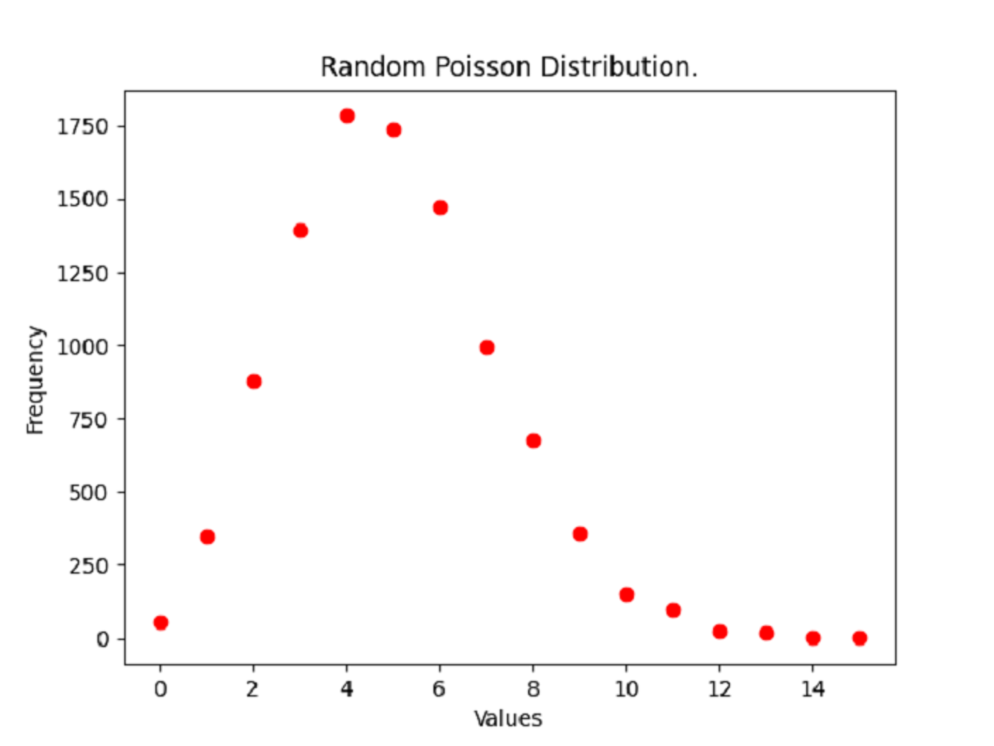
You first generate a NumPy array of ten thousand random samples from the Poisson distribution whose λ value is 5. NumPy’s unique() function then produces a frequency distribution by counting each unique sample value. You then plot the frequency of each individual value, and the plot’s shape proves that the ten thousand random samples conform to a Poisson distribution.
Conclusion
You’re now familiar with how pseudo-random number generation works and which random number generation features NumPy offers. You can use your new skills to generate random numbers both individually and as NumPy arrays. You know how to select random items, rows, and columns from an array and how to randomize them. Finally, you gained insight into how NumPy supports random selection from statistical distributions.
In this tutorial, you’ve learned:
- How computers perform pseudo-random number generation
- How to generate NumPy arrays of random numbers
- How to randomize NumPy arrays
- How to randomly select elements, rows, and columns from a NumPy array
- How to select random samples from the Poisson statistical distribution
If you’d like to continue exploring NumPy’s capabilities, then your next step could be to explore getting normally distributed random numbers. If you want even more, then you can take a look at the range of the Generator object’s statistical methods in the NumPy documentation.
Do you have an interesting example of using random numbers? Perhaps you have a card trick to entertain your fellow programmers with, or a lottery number predictor that can make us all rich. Share your ideas with the community in the comments below.
Free Bonus: Click here to download the sample code that shows you how to get random numbers with NumPy.