Watch Now This tutorial has a related video course created by the Real Python team. Watch it together with the written tutorial to deepen your understanding: Exploring the Python math Module
In this article, you’ll learn all about Python’s math module. Mathematical calculations are an essential part of most Python development. Whether you’re working on a scientific project, a financial application, or any other type of programming endeavor, you just can’t escape the need for math.
For straightforward mathematical calculations in Python, you can use the built-in mathematical operators, such as addition (+), subtraction (-), division (/), and multiplication (*). But more advanced operations, such as exponential, logarithmic, trigonometric, or power functions, are not built in. Does that mean you need to implement all of these functions from scratch?
Fortunately, no. Python provides a module specifically designed for higher-level mathematical operations: the math module.
By the end of this article, you’ll learn:
- What the Python
mathmodule is - How to use
mathmodule functions to solve real-life problems - What the constants of the
mathmodule are, including pi, tau, and Euler’s number - What the differences between built-in functions and
mathfunctions are - What the differences between
math,cmath, and NumPy are
A background in mathematics will be helpful here, but don’t worry if math isn’t your strong suit. This article will explain the basics of everything you need to know.
So let’s get started!
Free Download: Get a sample chapter from Python Tricks: The Book that shows you Python’s best practices with simple examples you can apply instantly to write more beautiful + Pythonic code.
Getting to Know the Python math Module
The Python math module is an important feature designed to deal with mathematical operations. It comes packaged with the standard Python release and has been there from the beginning. Most of the math module’s functions are thin wrappers around the C platform’s mathematical functions. Since its underlying functions are written in CPython, the math module is efficient and conforms to the C standard.
The Python math module offers you the ability to perform common and useful mathematical calculations within your application. Here are a few practical uses for the math module:
- Calculating combinations and permutations using factorials
- Calculating the height of a pole using trigonometric functions
- Calculating radioactive decay using the exponential function
- Calculating the curve of a suspension bridge using hyperbolic functions
- Solving quadratic equations
- Simulating periodic functions, such as sound and light waves, using trigonometric functions
Since the math module comes packaged with the Python release, you don’t have to install it separately. Using it is just a matter of importing the module:
>>> import math
You can import the Python math module using the above command. After importing, you can use it straightaway.
Constants of the math Module
The Python math module offers a variety of predefined constants. Having access to these constants provides several advantages. For one, you don’t have to manually hardcode them into your application, which saves you a lot of time. Plus, they provide consistency throughout your code. The module includes several famous mathematical constants and important values:
- Pi
- Tau
- Euler’s number
- Infinity
- Not a number (NaN)
In this section, you’ll learn about the constants and how to use them in your Python code.
Pi
Pi (π) is the ratio of a circle’s circumference (c) to its diameter (d):
π = c/d
This ratio is always the same for any circle.
Pi is an irrational number, which means it can’t be expressed as a simple fraction. Therefore, pi has an infinite number of decimal places, but it can be approximated as 22/7, or 3.141.
Interesting Fact: Pi is the most recognized and well-known mathematical constant in the world. It has its own celebration date, called Pi Day, which falls on March 14th (3/14).
You can access pi as follows:
>>> math.pi
3.141592653589793
As you can see, the pi value is given to fifteen decimal places in Python. The number of digits provided depends on the underlying C compiler. Python prints the first fifteen digits by default, and math.pi always returns a float value.
So what are some of the ways that pi can be useful to you? You can calculate the circumference of a circle using 2πr, where r is the radius of the circle:
>>> r = 3
>>> circumference = 2 * math.pi * r
>>> f"Circumference of a Circle = 2 * {math.pi:.4} * {r} = {circumference:.4}"
'Circumference of a Circle = 2 * 3.142 * 3 = 18.85'
You can use math.pi to calculate the circumference of a circle. You can also calculate the area of a circle using the formula πr² as follows:
>>> r = 5
>>> area = math.pi * r * r
>>> f"Area of a Circle = {math.pi:.4} * {r} * {r} = {area:.4}"
'Area of a Circle = 3.142 * 5 * 5 = 78.54'
You can use math.pi to calculate the area and the circumference of a circle. When you are doing mathematical calculations with Python and you come across a formula that uses π, it’s a best practice to use the pi value given by the math module instead of hardcoding the value.
Tau
Tau (τ) is the ratio of a circle’s circumference to its radius. This constant is equal to 2π, or roughly 6.28. Like pi, tau is an irrational number because it’s just pi times two.
Many mathematical expressions use 2π, and using tau instead can help simplify your equations. For example, instead of calculating the circumference of a circle with 2πr, we can substitute tau and use the simpler equation τr.
The use of tau as the circle constant, however, is still under debate. You have the freedom to use either 2π or τ as necessary.
You can use tau as below:
>>> math.tau
6.283185307179586
Like math.pi, math.tau returns fifteen digits and is a float value. You can use tau to calculate the circumference of a circle with τr, where r is the radius, as follows:
>>> r = 3
>>> circumference = math.tau * r
>>> f"Circumference of a Circle = {math.tau:.4} * {r} = {circumference:.4}"
'Circumference of a Circle = 6.283 * 3 = 18.85'
You can use math.tau in place of 2 * math.pi to tidy up equations that include the expression 2π.
Euler’s Number
Euler’s number (e) is a constant that is the base of the natural logarithm, a mathematical function that is commonly used to calculate rates of growth or decay. As with pi and tau, Euler’s number is an irrational number with infinite decimal places. The value of e is often approximated as 2.718.
Euler’s number is an important constant because it has many practical uses, such as calculating population growth over time or determining rates of radioactive decay. You can access Euler’s number from the math module as follows:
>>> math.e
2.718281828459045
As with math.pi and math.tau, the value of math.e is given to fifteen decimal places and is returned as a float value.
Infinity
Infinity can’t be defined by a number. Rather, it’s a mathematical concept representing something that is never-ending or boundless. Infinity can go in either direction, positive or negative.
You can use infinity in algorithms when you want to compare a given value to an absolute maximum or minimum value. The values of positive and negative infinity in Python are as follows:
>>> f"Positive Infinity = {math.inf}"
'Positive Infinity = inf'
>>> f"Negative Infinity = {-math.inf}"
'Negative Infinity = -inf'
Infinity is not a numerical value. Instead, it’s defined as math.inf. Python introduced this constant in version 3.5 as an equivalent to float("inf"):
>>> float("inf") == math.inf
True
Both float("inf") and math.inf represent the concept of infinity, making math.inf greater than any numerical value:
>>> x = 1e308
>>> math.inf > x
True
In the above code, math.inf is greater than the value of x, 10308 (the maximum size of a floating-point number), which is a double precision number.
Similarly, -math.inf is smaller than any value:
>>> y = -1e308
>>> y > -math.inf
True
Negative infinity is smaller than the value of y, which is -10308. No number can be greater than infinity or smaller than negative infinity. That’s why mathematical operations with math.inf don’t change the value of infinity:
>>> math.inf + 1e308
inf
>>> math.inf / 1e308
inf
As you can see, neither addition nor division changes the value of math.inf.
Not a Number (NaN)
Not a number, or NaN, isn’t really a mathematical concept. It originated in the computer science field as a reference to values that are not numeric. A NaN value can be due to invalid inputs, or it can indicate that a variable that should be numerical has been corrupted by text characters or symbols.
It’s always a best practice to check if a value is NaN. If it is, then it could lead to invalid values in your program. Python introduced the NaN constant in version 3.5.
You can observe the value of math.nan below:
>>> math.nan
nan
NaN is not a numerical value. You can see that the value of math.nan is nan, the same value as float("nan").
Arithmetic Functions
Number theory is a branch of pure mathematics, which is the study of natural numbers. Number theory usually deals with positive whole numbers or integers.
The Python math module provides functions that are useful in number theory as well as in representation theory, a related field. These functions allow you to calculate a range of important values, including the following:
- The factorials of a number
- The greatest common divisor of two numbers
- The sum of iterables
Find Factorials With Python factorial()
You may have seen mathematical expressions like 7! or 4! before. The exclamation marks don’t mean that the numbers are excited. Rather, “!” is the factorial symbol. Factorials are used in finding permutations or combinations. You can determine the factorial of a number by multiplying all whole numbers from the chosen number down to 1.
The following table shows the factorial values for 4, 6, and 7:
| Symbol | In Words | Expression | Result |
|---|---|---|---|
| 4! | Four factorial | 4 x 3 x 2 x 1 | 24 |
| 6! | Six factorial | 6 x 5 x 4 x 3 x 2 x 1 | 720 |
| 7! | Seven factorial | 7 x 6 x 5 x 4 x 3 x 2 x 1 | 5040 |
You can see from the table that 4!, or four factorial, gives the value 24 by multiplying the range of whole numbers from 4 to 1. Similarly, 6! and 7! give the values 720 and 5040, respectively.
You can implement a factorial function in Python using one of several tools:
forloops- Recursive functions
math.factorial()
First you are going to look at a factorial implementation using a for loop. This is a relatively straightforward approach:
def fact_loop(num):
    if num < 0:
        return 0
    if num == 0:
        return 1

    factorial = 1
    for i in range(1, num + 1):
        factorial = factorial * i
    return factorial
You can also use a recursive function to find the factorial. This is more complicated but also more elegant than using a for loop. You can implement the recursive function as follows:
def fact_recursion(num):
    if num < 0:
        return 0
    if num == 0:
        return 1

    return num * fact_recursion(num - 1)
Note: There is a limit to the recursion depth in Python, but that subject is outside the scope of this article.
The following example illustrates how you can use the for loop and recursive functions:
>>> fact_loop(7)
5040

>>> fact_recursion(7)
5040
Even though their implementations are different, their return values are the same.
However, implementing functions of your own just to get the factorial of a number is time consuming and inefficient. A better method is to use math.factorial(). Here’s how you can find the factorial of a number using math.factorial():
>>> math.factorial(7)
5040
This approach returns the desired output with a minimal amount of code.
factorial() accepts only positive integer values. If you try to input a negative value, then you will get a ValueError:
>>> math.factorial(-5)
Traceback (most recent call last):
  File "<stdin>", line 1, in <module>
ValueError: factorial() not defined for negative values
Inputting a negative value will result in a ValueError reading factorial() not defined for negative values.
factorial() doesn’t accept decimal numbers, either. It will give you a ValueError:
>>> math.factorial(4.3)
Traceback (most recent call last):
  File "<stdin>", line 1, in <module>
ValueError: factorial() only accepts integral values
Inputting a decimal value results in a ValueError reading factorial() only accepts integral values.
You can compare the execution times for each of the factorial methods using timeit():
>>> import timeit
>>> timeit.timeit("fact_loop(10)", globals=globals())
1.063997201999996

>>> timeit.timeit("fact_recursion(10)", globals=globals())
1.815312818999928

>>> timeit.timeit("math.factorial(10)", setup="import math")
0.10671788000001925
The sample above illustrates the results of timeit() for each of the three factorial methods.
timeit() executes one million loops each time it is run. The following table compares the execution times of the three factorial methods:
| Type | Execution Time |
|---|---|
| With loops | 1.0640 s |
| With recursion | 1.8153 s |
With factorial() |
0.1067 s |
As you can see from the execution times, factorial() is faster than the other methods. That’s because of its underlying C implementation. The recursion-based method is the slowest out of the three. Although you might get different timings depending on your CPU, the order of the functions should be the same.
Not only is factorial() faster than the other methods, but it’s also more stable. When you implement your own function, you have to explicitly code for disaster cases such as handling negative or decimal numbers. One mistake in the implementation could lead to bugs. But when using factorial(), you don’t have to worry about disaster cases because the function handles them all. Therefore, it’s a best practice to use factorial() whenever possible.
Find the Ceiling Value With ceil()
math.ceil() will return the smallest integer value that is greater than or equal to the given number. If the number is a positive or negative decimal, then the function will return the next integer value greater than the given value.
For example, an input of 5.43 will return the value 6, and an input of -12.43 will return the value -12. math.ceil() can take positive or negative real numbers as input values and will always return an integer value.
When you input an integer value to ceil(), it will return the same number:
>>> math.ceil(6)
6
>>> math.ceil(-11)
-11
math.ceil() always returns the same value when an integer is given as input. To see the true nature of ceil(), you have to input decimal values:
>>> math.ceil(4.23)
5
>>> math.ceil(-11.453)
-11
When the value is positive (4.23), the function returns the next integer greater than the value (5). When the value is negative (-11.453), the function likewise returns the next integer greater than the value (-11).
The function will return a TypeError if you input a value that is not a number:
>>> math.ceil("x")
Traceback (most recent call last):
  File "<stdin>", line 1, in <module>
TypeError: must be real number, not str
You must input a number to the function. If you try to input any other value, then you will get a TypeError.
Find the Floor Value With floor()
floor() will return the closest integer value that is less than or equal to the given number. This function behaves opposite to ceil(). For example, an input of 8.72 will return 8, and an input of -12.34 will return -13. floor() can take either positive or negative numbers as input and will return an integer value.
If you input an integer value, then the function will return the same value:
>>> math.floor(4)
4
>>> math.floor(-17)
-17
As with ceil(), when the input for floor() is an integer, the result will be the same as the input number. The output only differs from the input when you input decimal values:
>>> math.floor(5.532)
5
>>> math.floor(-6.432)
-7
When you input a positive decimal value (5.532), it will return the closest integer that is less than the input number (5). If you input a negative number (-6.432), then it will return the next lowest integer value (-7).
If you try to input a value that is not a number, then the function will return a TypeError:
>>> math.floor("x")
Traceback (most recent call last):
  File "<stdin>", line 1, in <module>
TypeError: must be real number, not str
You can’t give non-number values as input to ceil(). Doing so will result in a TypeError.
Truncate Numbers With trunc()
When you get a number with a decimal point, you might want to keep only the integer part and eliminate the decimal part. The math module has a function called trunc() which lets you do just that.
Dropping the decimal value is a type of rounding. With trunc(), negative numbers are always rounded upward toward zero and positive numbers are always rounded downward toward zero.
Here is how the trunc() function rounds off positive or negative numbers:
>>> math.trunc(12.32)
12
>>> math.trunc(-43.24)
-43
As you can see, 12.32 is rounded downwards towards 0, which gives the result 12. In the same way, -43.24 is rounded upwards towards 0, which gives the value -43. trunc() always rounds towards zero regardless of whether the number is positive or negative.
When dealing with positive numbers, trunc() behaves the same as floor():
>>> math.trunc(12.32) == math.floor(12.32)
True
trunc() behaves the same as floor() for positive numbers. As you can see, the return value of both functions is the same.
When dealing with negative numbers, trunc() behaves the same as ceil():
>>> math.trunc(-43.24) == math.ceil(-43.24)
True
When the number is negative, floor() behaves the same as ceil(). The return values of both functions are the same.
Find the Closeness of Numbers With Python isclose()
In certain situations—particularly in the data science field—you may need to determine whether two numbers are close to each other. But to do so, you first need to answer an important question: How close is close? In other words, what is the definition of close?
Well, Merriam-Webster will tell you that close means “near in time, space, effect, or degree.” Not very helpful, is it?
For example, take the following set of numbers: 2.32, 2.33, and 2.331. When you measure closeness by two decimal points, 2.32 and 2.33 are close. But in reality, 2.33 and 2.331 are closer. Closeness, therefore, is a relative concept. You can’t determine closeness without some kind of threshold.
Fortunately, the math module provides a function called isclose() that lets you set your own threshold, or tolerance, for closeness. It returns True if two numbers are within your established tolerance for closeness and otherwise returns False.
Let’s check out how to compare two numbers using the default tolerances:
- Relative tolerance, or rel_tol, is the maximum difference for being considered “close” relative to the magnitude of the input values. This is the percentage of tolerance. The default value is 1e-09 or 0.000000001.
- Absolute tolerance, or abs_tol, is the maximum difference for being considered “close” regardless of the magnitude of the input values. The default value is 0.0.
isclose() will return True when the following condition is satisfied:
abs(a-b) <= max(rel_tol * max(abs(a), abs(b)), abs_tol).
isclose uses the above expression to determine the closeness of two numbers. You can substitute your own values and observe whether any two numbers are close.
In the following case, 6 and 7 aren’t close:
>>> math.isclose(6, 7)
False
The numbers 6 and 7 aren’t considered close because the relative tolerance is set for nine decimal places. But if you input 6.999999999 and 7 under the same tolerance, then they are considered close:
>>> math.isclose(6.999999999, 7)
True
You can see that the value 6.999999999 is within nine decimal places of 7. Therefore, based on the default relative tolerance, 6.999999999 and 7 are considered close.
You can adjust the relative tolerance however you want depending on your need. If you set rel_tol to 0.2, then 6 and 7 are considered close:
>>> math.isclose(6, 7, rel_tol=0.2)
True
You can observe that 6 and 7 are close now. This is because they are within 20% of each other.
As with rel_tol, you can adjust the abs_tol value according to your needs. To be considered close, the difference between the input values must be less than or equal to the absolute tolerance value. You can set the abs_tol as follows:
>>> math.isclose(6, 7, abs_tol=1.0)
True
>>> math.isclose(6, 7, abs_tol=0.2)
False
When you set the absolute tolerance to 1, the numbers 6 and 7 are close because the difference between them is equal to the absolute tolerance. However, in the second case, the difference between 6 and 7 is not less than or equal to the established absolute tolerance of 0.2.
You can use the abs_tol for very small values:
>>> math.isclose(1, 1.0000001, abs_tol=1e-08)
False
>>> math.isclose(1, 1.00000001, abs_tol=1e-08)
True
As you can see, you can determine the closeness of very small numbers with isclose. A few special cases regarding closeness can be illustrated using nan and inf values:
>>> math.isclose(math.nan, 1e308)
False
>>> math.isclose(math.nan, math.nan)
False

>>> math.isclose(math.inf, 1e308)
False
>>> math.isclose(math.inf, math.inf)
True
You can see from the above examples that nan is not close to any value, not even to itself. On the other hand, inf is not close to any numerical values, not even to very large ones, but it is close to itself.
Power Functions
The power function takes any number x as input, raises x to some power n, and returns xn as output. Python’s math module provides several power-related functions. In this section, you’ll learn about power functions, exponential functions, and square root functions.
Calculate the Power of a Number With pow()
Power functions have the following formula where the variable x is the base, the variable n is the power, and a can be any constant:

In the formula above, the value of the base x is raised to the power of n.
You can use math.pow() to get the power of a number. There is a built-in function, pow(), that is different from math.pow(). You will learn the difference later in this section.
math.pow() takes two parameters as follows:
>>> math.pow(2, 5)
32.0
>>> math.pow(5, 2.4)
47.59134846789696
The first argument is the base value and the second argument is the power value. You can give an integer or a decimal value as input and the function always returns a float value. There are some special cases defined in math.pow().
When the base 1 is raised to the power of any number n, it gives the result 1.0:
>>> math.pow(1.0, 3)
1.0
When you raise base value 1 to any power value, you will always get 1.0 as the result. Likewise, any base number raised to the power of 0 gives the result 1.0:
>>> math.pow(4, 0.0)
1.0
>>> math.pow(-4, 0.0)
1.0
As you can see, any number raised to the power of 0 will give 1.0 as the result. You can see that result even if the base is nan:
>>> math.pow(math.nan, 0.0)
1.0
Zero raised to the power of any positive number will give 0.0 as the result:
>>> math.pow(0.0, 2)
0.0
>>> math.pow(0.0, 2.3)
0.0
But if you try to raise 0.0 to a negative power, then the result will be a ValueError:
>>> math.pow(0.0, -2)
Traceback (most recent call last):
  File "<stdin>", line 1, in <module>
ValueError: math domain error
The ValueError only occurs when the base is 0. If the base is any other number except 0, then the function will return a valid power value.
Apart from math.pow(), there are two built-in ways of finding the power of a number in Python:
x ** ypow()
The first option is straightforward. You may have used it a time or two already. The return type of the value is determined by the inputs:
>>> 3 ** 2
9
>>> 2 ** 3.3
9.849155306759329
When you use integers, you get an integer value. When you use decimal values, the return type changes to a decimal value.
The second option is a versatile built-in function. You don’t have to use any imports to use it. The built-in pow() method has three parameters:
- The base number
- The power number
- The modulus number
The first two parameters are mandatory, whereas the third parameter is optional. You can input integers or decimal numbers and the function will return the appropriate result based on the input:
>>> pow(3, 2)
9
>>> pow(2, 3.3)
9.849155306759329
The built-in pow() has two required arguments that work the same as the base and power in the x ** y syntax. pow() also has a third parameter that is optional: modulus. This parameter is often used in cryptography. Built-in pow() with the optional modulus parameter is equivalent to the equation (x ** y) % z. The Python syntax looks like this:
>>> pow(32, 6, 5)
4
>>> (32 ** 6) % 5 == pow(32, 6, 5)
True
pow() raises the base (32) to the power (6), and then the result value is modulo divided by the modulus number (5). In this case, the result is 4. You can substitute your own values and see that both pow() and the given equation provide the same results.
Even though all three methods of calculating power do the same thing, there are some implementation differences between them. The execution times for each method are as follows:
>>> timeit.timeit("10 ** 308")
1.0078728999942541

>>> timeit.timeit("pow(10, 308)")
1.047615700008464

>>> timeit.timeit("math.pow(10, 308)", setup="import math")
0.1837239999877056
The following table compares the execution times of the three methods as measured by timeit():
| Type | Execution Time |
|---|---|
x ** y |
1.0079 s |
pow(x, y) |
1.0476 s |
math.pow(x, y) |
0.1837 s |
You can observe from the table that math.pow() is faster than the other methods and built-in pow() is the slowest.
The reason behind the efficiency of math.pow() is the way that it’s implemented. It relies on the underlying C language. On the other hand, pow() and x ** y use the input object’s own implementation of the ** operator. However, math.pow() can’t handle complex numbers (which will be explained in a later section), whereas pow() and ** can.
Find the Natural Exponent With exp()
You learned about power functions in the previous section. With exponential functions, things are a bit different. Instead of the base being the variable, power becomes the variable. It looks something like this:

Here a can be any constant, and x, which is the power value, becomes the variable.
So what’s so special about exponential functions? The value of the function grows rapidly as the x value increases. If the base is greater than 1, then the function continuously increases in value as x increases. A special property of exponential functions is that the slope of the function also continuously increases as x increases.
You learned about the Euler’s number in a previous section. It is the base of the natural logarithm. It also plays a role with the exponential function. When Euler’s number is incorporated into the exponential function, it becomes the natural exponential function:

This function is used in many real-life situations. You may have heard of the term exponential growth, which is often used in relation to human population growth or rates of radioactive decay. Both of these can be calculated using the natural exponential function.
The Python math module provides a function, exp(), that lets you calculate the natural exponent of a number. You can find the value as follows:
>>> math.exp(21)
1318815734.4832146
>>> math.exp(-1.2)
0.30119421191220214
The input number can be positive or negative, and the function always returns a float value. If the number is not a numerical value, then the method will return a TypeError:
>>> math.exp("x")
Traceback (most recent call last):
  File "<stdin>", line 1, in <module>
TypeError: must be real number, not str
As you can see, if the input is a string value, then the function returns a TypeError reading must be real number, not str.
You can also calculate the exponent using the math.e ** x expression or by using pow(math.e, x). The execution times of these three methods are as follows:
>>> timeit.timeit("math.e ** 308", setup="import math")
0.17853009998701513

>>> timeit.timeit("pow(math.e, 308)", setup="import math")
0.21040189999621361

>>> timeit.timeit("math.exp(308)", setup="import math")
0.125878200007719
The following table compares the execution times of the above methods as measured by timeit():
| Type | Execution Time |
|---|---|
e ** x |
0.1785 s |
pow(e, x) |
0.2104 s |
math.exp(x) |
0.1259 s |
You can see that math.exp() is faster than the other methods and pow(e, x) is the slowest. This is the expected behavior because of the underlying C implementation of the math module.
It’s also worth noting that e ** x and pow(e, x) return the same values, but exp() returns a slightly different value. This is due to implementation differences. Python documentation notes that exp() is more accurate than the other two methods.
Practical Example With exp()
Radioactive decay happens when an unstable atom loses energy by emitting ionizing radiation. The rate of radioactive decay is measured using half-life, which is the time it takes for half the amount of the parent nucleus to decay. You can calculate the decay process using the following formula:

You can use the above formula to calculate the remaining quantity of a radioactive element after a certain number of years. The variables of the given formula are as follows:
- N(0) is the initial quantity of the substance.
- N(t) is the quantity that still remains and has not yet decayed after a time (t).
- T is the half-life of the decaying quantity.
- e is Euler’s number.
Scientific research has identified the half-lives of all radioactive elements. You can substitute values to the equation to calculate the remaining quantity of any radioactive substance. Let’s try that now.
The radioisotope strontium-90 has a half-life of 38.1 years. A sample contains 100 mg of Sr-90. You can calculate the remaining milligrams of Sr-90 after 100 years:
>>> half_life = 38.1
>>> initial = 100
>>> time = 100
>>> remaining = initial * math.exp(-0.693 * time / half_life)
>>> f"Remaining quantity of Sr-90: {remaining}"
'Remaining quantity of Sr-90: 16.22044604811303'
As you can see, the half-life is set to 38.1 and the duration is set to 100 years. You can use math.exp to simplify the equation. By substituting the values to the equation you can find that, after 100 years, 16.22mg of Sr-90 remains.
Logarithmic Functions
Logarithmic functions can be considered the inverse of exponential functions. They are denoted in the following form:

Here a is the base of the logarithm, which can be any number. You learned about exponential functions in a previous section. Exponential functions can be expressed in the form of logarithmic functions and vice versa.
Python Natural Log With log()
The natural logarithm of a number is its logarithm to the base of the mathematical constant e, or Euler’s number:

As with the exponential function, natural log uses the constant e. It’s generally depicted as f(x) = ln(x), where e is implicit.
You can use the natural log in the same way that you use the exponential function. It’s used to calculate values such as the rate of population growth or the rate of radioactive decay in elements.
log() has two arguments. The first one is mandatory and the second one is optional. With one argument you can get the natural log (to the base e) of the input number:
>>> math.log(4)
1.3862943611198906
>>> math.log(3.4)
1.2237754316221157
However, the function returns a ValueError if you input a non-positive number:
>>> math.log(-3)
Traceback (most recent call last):
  File "<stdin>", line 1, in <module>
ValueError: math domain error
As you can see, you can’t input a negative value to log(). This is because log values are undefined for negative numbers and zero.
With two arguments, you can calculate the log of the first argument to the base of the second argument:
>>> math.log(math.pi, 2)
1.651496129472319
>>> math.log(math.pi, 5)
0.711260668712669
You can see how the value changes when the log base is changed.
Understand log2() and log10()
The Python math module also provides two separate functions that let you calculate the log values to the base of 2 and 10:
log2()is used to calculate the log value to the base 2.log10()is used to calculate the log value to the base 10.
With log2() you can get the log value to the base 2:
>>> math.log2(math.pi)
1.6514961294723187
>>> math.log(math.pi, 2)
1.651496129472319
Both functions have the same objective, but the Python documentation notes that log2() is more accurate than using log(x, 2).
You can calculate the log value of a number to base 10 with log10():
>>> math.log10(math.pi)
0.4971498726941338
>>> math.log(math.pi, 10)
0.4971498726941338
The Python documentation also mentions that log10() is more accurate than log(x, 10) even though both functions have the same objective.
Practical Example With Natural Log
In a previous section, you saw how to use math.exp() to calculate the remaining amount of a radioactive element after a certain period of time. With math.log(), you can find the half-life of an unknown radioactive element by measuring the mass at an interval. The following equation can be used to calculate the half-life of a radioactive element:

By rearranging the radioactive decay formula, you can make the half-life (T) the subject of the formula. The variables of the given formula are as follows:
- T is the half-life of the decaying quantity.
- N(0) is the initial quantity of the substance.
- N(t) is the quantity that remains and has not yet decayed after a period of time (t).
- ln is the natural log.
You can substitute the known values to the equation to calculate the half-life of a radioactive substance.
For example, imagine you are studying an unidentified radioactive element sample. When it was discovered 100 years ago, the sample size was 100mg. After 100 years of decay, only 16.22mg is remaining. Using the formula above, you can calculate the half-life of this unknown element:
>>> initial = 100
>>> remaining = 16.22
>>> time = 100
>>> half_life = (-0.693 * time) / math.log(remaining / initial)
>>> f"Half-life of the unknown element: {half_life}"
'Half-life of the unknown element: 38.09942398335152'
You can see that the unknown element has a half-life of roughly 38.1 years. Based on this information, you can identify the unknown element as strontium-90.
Other Important math Module Functions
The Python math module has many useful functions for mathematical calculations, and this article only covered a few of them in depth. In this section, you will briefly learn about some of the other important functions available in the math module.
Calculate the Greatest Common Divisor
The greatest common divisor (GCD) of two positive numbers is the largest positive integer that divides both numbers without a remainder.
For example, the GCD of 15 and 25 is 5. You can divide both 15 and 25 by 5 without any remainder. There is no greater number that does the same. If you take 15 and 30, then the GCD is 15 because both 15 and 30 can be divided by 15 without a remainder.
You don’t have to implement your own functions to calculate GCD. The Python math module provides a function called math.gcd() that allows you to calculate the GCD of two numbers. You can give positive or negative numbers as input, and it returns the appropriate GCD value. You can’t input a decimal number, however.
Calculate the Sum of Iterables
If you ever want to find the sum of the values of an iterable without using a loop, then math.fsum() is probably the easiest way to do so. You can use iterables such as arrays, tuples, or lists as input and the function returns the sum of the values. A built-in function called sum() lets you calculate the sum of iterables as well, but fsum() is more accurate than sum(). You can read more about that in the documentation.
Calculate the Square Root
The square root of a number is a value that, when multiplied by itself, gives the number. You can use math.sqrt() to find the square root of any positive real number (integer or decimal). The return value is always a float value. The function will throw a ValueError if you try to enter a negative number.
Convert Angle Values
In real-life scenarios as well as in mathematics, you often come across instances where you have to measure angles to perform calculations. Angles can be measured either by degrees or by radians. Sometimes you have to convert degrees to radians and vice versa. The math module provides functions that let you do so.
If you want to convert degrees to radians, then you can use math.radians(). It returns the radian value of the degree input. Likewise, if you want to convert radians to degrees, then you can use math.degrees().
Calculate Trigonometric Values
Trigonometry is the study of triangles. It deals with the relationship between angles and the sides of a triangle. Trigonometry is mostly interested in right-angled triangles (in which one internal angle is 90 degrees), but it can also be applied to other types of triangles. The Python math module provides very useful functions that let you perform trigonometric calculations.
You can calculate the sine value of an angle with math.sin(), the cosine value with math.cos(), and the tangent value with math.tan(). The math module also provides functions to calculate arc sine with math.asin(), arc cosine with math.acos(), and arc tangent with math.atan(). Finally, you can calculate the hypotenuse of a triangle using math.hypot().
New Additions to the math Module in Python 3.8
With the release of Python version 3.8, a few new additions and changes have been made to the math module. The new additions and changes are as follows:
-
comb(n, k)returns the number of ways to choose k items from n items without repetition and without particular order. -
perm(n, k)returns the number of ways to choose k items from n items without repetition and with order. -
isqrt()returns the integer square root of a non-negative integer. -
prod()calculates the product of all of the elements in the input iterable. As withfsum(), this method can take iterables such as arrays, lists, or tuples. -
dist()returns the Euclidean distance between two points p and q, each given as a sequence (or iterable) of coordinates. The two points must have the same dimension. -
hypot()now handles more than two dimensions. Previously, it supported a maximum of two dimensions.
cmath vs math
A complex number is a combination of a real number and an imaginary number. It has the formula of a + bi, where a is the real number and bi is the imaginary number. Real and imaginary numbers can be explained as follows:
- A real number is literally any number you can think of.
- An imaginary number is a number that gives a negative result when squared.
A real number can be any number. For example, 12, 4.3, -19.0 are all real numbers. Imaginary numbers are shown as i. The following image shows an example of a complex number:
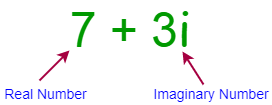
In the example above, 7 is the real number and 3i is the imaginary number. Complex numbers are mostly used in geometry, calculus, scientific calculations, and especially in electronics.
The functions of the Python math module aren’t equipped to handle complex numbers. However, Python provides a different module that can specifically deal with complex numbers, the cmath module. The Python math module is complemented by the cmath module, which implements many of the same functions but for complex numbers.
You can import the cmath module as follows:
>>> import cmath
Since the cmath module is also packaged with Python, you can import it the same way you imported the math module. Before you work with the cmath module, you have to know how to define a complex number. You can define a complex number as follows:
>>> c = 2 + 3j
>>> c
(2+3j)

>>> type(c)
<class 'complex'>
As you can see, you can determine that a number is indeed complex by using type().
Note: In mathematics, the imaginary unit is usually denoted i. In some fields, it’s more customary to use j for the same thing. In Python, you use j to denote imaginary numbers.
Python also provides a special built-in function called complex() that lets you create complex numbers. You can use complex() as follows:
>>> c = complex(2, 3)
>>> c
(2+3j)

>>> type(c)
<class 'complex'>
You can use either method to create complex numbers. You can also use the cmath module to calculate mathematical functions for complex numbers as follows:
>>> cmath.sqrt(c)
(1.8581072140693775+0.6727275964137814j)

>>> cmath.log(c)
(1.3622897515267103+0.6947382761967031j)

>>> cmath.exp(c)
(-16.091399670844+12.02063434789931j)
This example shows you how to calculate the square root, logarithmic value, and exponential value of a complex number. You can read the documentation if you want to learn more about the cmath module.
NumPy vs math
Several notable Python libraries can be used for mathematical calculations. One of the most prominent libraries is Numerical Python, or NumPy. It is mainly used in scientific computing and in data science fields. Unlike the math module, which is part of the standard Python release, you have to install NumPy in order to work with it.
The heart of NumPy is the high-performance N-dimensional (multidimensional) array data structure. This array allows you to perform mathematical operations on an entire array without looping over the elements. All of the functions in the library are optimized to work with the N-dimensional array objects.
Both the math module and the NumPy library can be used for mathematical calculations. NumPy has several similarities with the math module. NumPy has a subset of functions, similar to math module functions, that deal with mathematical calculations. Both NumPy and math provide functions that deal with trigonometric, exponential, logarithmic, hyperbolic and arithmetic calculations.
There are also several fundamental differences between math and NumPy. The Python math module is geared more towards working with scalar values, whereas NumPy is better suited for working with arrays, vectors, and even matrices.
When working with scalar values, math module functions can be faster than their NumPy counterparts. This is because the NumPy functions convert the values to arrays under the hood in order to perform calculations on them. NumPy is much faster when working with N-dimensional arrays because of the optimizations for them. Except for fsum() and prod(), the math module functions can’t handle arrays.
Conclusion
In this article, you learned about the Python math module. The module provides useful functions for performing mathematical calculations that have many practical applications.
In this article you’ve learned:
- What the Python
mathmodule is - How to use
mathfunctions with practical examples - What the constants of the
mathmodule, including pi, tau, and Euler’s number are - What the differences between built-in functions and
mathfunctions are - What the differences between
math,cmath, and NumPy are
Understanding how to use the math functions is the first step. Now it’s time to start applying what you learned to real-life situations. If you have any questions or comments, then please leave them in the comments section below.
Watch Now This tutorial has a related video course created by the Real Python team. Watch it together with the written tutorial to deepen your understanding: Exploring the Python math Module