Watch Now This tutorial has a related video course created by the Real Python team. Watch it together with the written tutorial to deepen your understanding: Mazes in Python: Build, Visualize, Store, and Solve
If you’re up for a little challenge and would like to take your programming skills to the next level, then you’ve come to the right place! In this hands-on tutorial, you’ll practice object-oriented programming, among several other good practices, while building a cool maze solver project in Python.
From reading a maze from a binary file, to visualizing it using scalable vector graphics (SVG), to finding the shortest path from the entrance to the exit, you’ll go step by step through the guided process of building a complete and working project.
In this tutorial, you’ll learn how to:
- Use an object-oriented approach to represent the maze in memory
- Define a specialized binary file format to store the maze on disk
- Transform the maze into a traversable weighted graph
- Use graph search algorithms in the NetworkX library to find the solution
- Visualize the maze and its solution using scalable vector graphics (SVG)
Click the link below to download the complete source code for this project, along with the supporting materials, which include a few sample mazes:
Free Download: Click here to download the source code and supporting materials that you’ll use to build a maze solver in Python.
Demo: Python Maze Solver
At the end of this tutorial, you’ll have a command-line maze solver that can load your maze from a binary file and show its solution in the web browser:
You’ll learn how to build your own mazes like this from scratch and save them on disk. In the meantime, feel free to grab one of the sample mazes from the supporting materials. Now, get ready to dive in!
Project Overview
Take a glimpse at the expected file structure of your project. Once finished, your project’s file and directory tree will look as follows:
maze-solver/
│
├── mazes/
│   ├── labyrinth.maze
│   ├── miniature.maze
│   └── pacman.maze
│
├── src/
│   │
│   └── maze_solver/
│       │
│       ├── graphs/
│       │   ├── __init__.py
│       │   ├── converter.py
│       │   └── solver.py
│       │
│       ├── models/
│       │   ├── __init__.py
│       │   ├── border.py
│       │   ├── edge.py
│       │   ├── maze.py
│       │   ├── role.py
│       │   ├── solution.py
│       │   └── square.py
│       │
│       ├── persistence/
│       │   ├── __init__.py
│       │   ├── file_format.py
│       │   └── serializer.py
│       │
│       ├── view/
│       │   ├── __init__.py
│       │   ├── decomposer.py
│       │   ├── primitives.py
│       │   └── renderer.py
│       │
│       ├── __init__.py
│       └── __main__.py
│
├── pyproject.toml
└── requirements.txt
Yes, that’s a lot of files, but don’t worry! Most of them are fairly short, and some contain only a few lines of code. This helps keep things organized and makes the individual pieces reusable, letting you compose them in new ways. Such granularity also plays an important role in Python projects with larger codebases by avoiding the notorious circular dependency error that you might encounter if various parts of the code were in one big file.
The mazes/ subfolder is home to a few binary files with sample data that you’re going to use in this tutorial. You can get these files, along with the final source code and snapshots of the individual steps, by downloading the supporting materials:
Free Download: Click here to download the source code and supporting materials that you’ll use to build a maze solver in Python.
The src/ subfolder contains your Python modules and packages for the maze solver project. The maze_solver package consists of several subpackages that group logically related code fragments, including:
graphs: The traversal and conversion of the maze to a graph representationmodels: The building blocks of the maze and its solutionpersistence: A custom binary file format for persistent maze storageview: The visualization of the graph with scalable vector graphics
You’ll also find the special __main__.py file, which makes the enclosing package runnable so that you can execute it directly from the command line using Python’s -m option:
$ python -m maze_solver /path/to/sample.maze
When launched like this, the package reads the specified file with your maze. After solving the maze, it renders the solution into an SVG format embedded in a temporary HTML file. The file gets automatically opened in your default web browser. You can also run the same Python code using a shortcut command:
$ solve /path/to/sample.maze
It’ll work as long the solve command isn’t already taken or aliased by another program.
Finally, pyproject.toml provides your project’s configuration, metadata, and dependencies defined in the TOML format. The project only depends on one external library, which you’ll use to find the shortest path in the maze represented as a graph.
Next up, you’ll review a list of relevant resources that might become your savior in case you get stuck at any point. Also, remember the supporting materials, which contain a snapshot of each finished step. Along the way, you can compare your progress to the relevant step to ensure that you’re on the right track.
Prerequisites
This tutorial will best suit intermediate Python developers who’d like to practice object-oriented programming (OOP) while building a cool project. Throughout this tutorial, you’ll be using several neat features of modern Python, so make sure you’re on Python 3.10 or later. Also, it might be worth brushing up on the following topics before you dive in:
- Assignment expressions
- Bitwise operators
- Class methods
- Data classes
- Enum
typing.NamedTuple- Structural pattern matching
- Type hints
Note that you don’t need to be an expert in any of these areas to follow along with the tutorial, as it’ll guide you through the steps involved. In fact, a key aspect of your learning experience will be seeing these features in a practical context.
With that out of the way, you can move on to your project!
Step 1: Lay the Groundwork for the Project
The first step to writing any code starts on paper. Therefore, you’ll now take a step back to figure out what problem you’re solving and how you’re going to approach it. You’ll begin by narrowing down the design requirements for your maze.
Define the Problem Constraints
Mazes come in different shapes and forms, but you’ll concentrate on one kind that you’d find in a typical maze-puzzle video game from the early 1980s, like Boulder Dash or Sokoban. For example, the following maze was inspired by the classic Pac-Man game:
This maze is enclosed in a rectangle comprising a grid of square cells that form passages along straight lines. Therefore, paths in your maze will only be vertical or horizontal rather than diagonal or circular, for example, and each cell will be one unit wide. This will become important for calculating and comparing the distances later.
Note: You can give your maze any shape by surrounding it with empty squares marked as exterior to form an open space. However, you might want to align the maze’s edges with the enclosing rectangle to save some memory.
An additional restriction that you’ll impose on your maze is that it must have exactly one entrance and exactly one exit, both of which should occupy distinct cells. A few alternative paths can connect them, including paths with cycles that lead back to a place you’ve already visited.
Solving the maze means finding a path leading from the entrance to the exit. Each solution should include acyclic paths. In other words, a single path location should only be traversed once without backtracking. You also want to consider only the shortest paths while disregarding less optimal, meandering ones. However, defining the shortest distance is subject to interpretation, as you’ll find out later in this tutorial.
Later, you’ll introduce enemies and rewards to the maze so that your hypothetical player can collect extra points and avoid obstacles. But how do you actually find the way out of the maze?
Well, mazes are a perfect example of graph theory in action. As it turns out, you can represent your maze with an undirected graph consisting of nodes and edges connecting them. Each node or vertex is where two or more paths intersect, while edges are the connections between those intersections:
Apart from nodes representing the intersections and dead ends in the maze, there are a few extra nodes in the graph above that capture the presence of enemies and rewards. By associating numeric weights with edges that pass through them, you can influence the cost of the given connection. Later, you’ll add nodes for corners to make plotting the path from the entrance to the exit a tad bit easier.
Note: Strictly speaking, the graph corresponding to a maze can be a more specialized type known as a multigraph when it has two or more parallel edges that connect neighboring nodes.
It’s worth noting that you can draw the same graph in different ways without changing its underlying structure. For example, you could draw all edges as straight lines, let them cross each other, or arrange the nodes in a certain pattern.
Mathematically, a graph is nothing more than a set of nodes and edges, which you can lay out in any order and locations you like. Therefore, transforming the maze into a graph is an irreversible process resulting in losing some information about its visual features. At the same time, a graph is a remarkably convenient representation for finding the shortest path in the maze.
In this tutorial, you won’t be implementing any graph traversal algorithms, such as the depth-first search (DFS), breadth-first search (BFS), or Dijkstra’s algorithm for finding the shortest path. Instead, you’ll leverage the excellent NetworkX library, which already implements these and more algorithms, to do the heavy lifting for you.
Now that you’ve clarified the problem at hand, you can start thinking about how to approach it from a technical perspective. It’s time to lay the groundwork for some Python code!
Scaffold the Project Structure
Use your favorite code editor or a cloud-based IDE to create a new Python project while specifying an isolated virtual environment for its dependencies. The minimum interpreter version required for this project is Python 3.10 due to a few syntactic constructs introduced in that release, which you’ll be using. If you can, consider switching to a more recent release for better performance and other improvements.
Note: You may use pyenv to manage multiple Python versions on your computer.
Once you have the project set up in your editor, scaffold the initial folder structure with these two nested Python packages, both of which should be empty at the moment:
maze-solver/
│
├── src/
│   │
│   └── maze_solver/
│       │
│       ├── models/
│       │   └── __init__.py
│       │
│       └── __init__.py
│
└── pyproject.toml
By placing the project’s root package under the src/ subfolder, you follow the so-called src layout convention for organizing files in a project. Note that the pyproject.toml file should live outside of the src/ subfolder.
The alternative is a flat layout with all files in the same folder. You can read about their differences in the official Python Packaging User Guide. In a nutshell, the src layout is preferred for larger projects because it allows you to better separate the project code from other files, such as tests.
While the project’s name is maze-solver with a hyphen (-), you named the corresponding Python package using an underscore character (_) to form a valid Python identifier, which follows the same rules as variable names. The rules for naming a Python project, or a distribution package in slightly more technical terms, are more liberal. If you’re curious enough, you can check PEP 508 to find the regular expression that validates these names.
To install your project in an active virtual environment, you’ll need to specify the minimum required configuration in the TOML file, such as the name and version of your project. Go ahead and open your pyproject.toml file now, and then paste the following content into it:
# pyproject.toml

[build-system]
requires = ["setuptools>=64.0.0", "wheel"]
build-backend = "setuptools.build_meta"

[project]
name = "maze-solver"
version = "1.0.0"
It’s a pretty standard configuration and a good starting point for most Python projects and libraries. Note that you don’t have to explicitly state what folder layout your project is following because the build tools like setuptools will automatically find your Python source code.
If you’re planning to publish your package on PyPI, then you should pick a globally unique name that won’t conflict with an existing Python distribution package. Otherwise, you have a fair amount of freedom in choosing your project name.
After you’ve saved your changes in the pyproject.toml file, you can install maze-solver with pip by running the following command from the root directory of your project:
(venv) $ python -m pip install --editable .
During the development of a src-layout project, it’s advisable to use the --editable flag or its -e alias to ensure that any changes you make to your code are immediately reflected in the virtual environment. Otherwise, you’d have to manually reinstall the package each time you edit the code.
Note: If you run into an error about not being able to install the directory in editable mode due to a missing setup.py or setup.cfg file, then you may need to upgrade pip itself:
(venv) $ python -m pip install --upgrade pip
Projects based on pyproject.toml support editable installs through PEP 660, which was implemented in pip starting from version 21.3.
To confirm that you’ve successfully installed the maze_solver package in your virtual environment, head over to the interactive Python REPL and try importing the package:
>>> import maze_solver
If everything works fine, then you shouldn’t see any output or error messages after running the line of code above. Otherwise, you’ll immediately get a ModuleNotFoundError.
Great! With the scaffolded Python project in place, you can now proceed to coding an object-oriented representation of the maze.
Step 2: Represent the Maze Using an Object-Oriented Approach
At this point, you know what kind of maze you’ll be solving and have a good idea of the best data structure to represent it with.
In this step, you’ll use a top-down approach to conceptually decompose the maze into a set of basic elements. One by one, you’ll implement those elements as objects and combine them to represent the complete maze. By the end of this step, you’ll be able to build any maze you like, including virtual replicas of real-world hedge mazes, maize mazes, or even ice mazes that can be found in amusement parks around the world!
Identify the Building Blocks of the Maze
For the purpose of this tutorial, you can think of the maze as a rectangular grid of uniform squares arranged in rows and columns. Each square has the same width and height and a piece of border around it. Squares can additionally play specific roles in the maze to make it more interesting. For example, some of them can represent obstacles like walls or enemies, while others can represent rewards.
To avoid tight coupling between your building blocks, which could manifest itself through the circular import error mentioned earlier, you’re going to put the individual classes in separate files. Go ahead and create the following four Python module placeholders in the models package:
maze-solver/
│
├── src/
│   │
│   └── maze_solver/
│       │
│       ├── models/
│       │   ├── __init__.py
│       │   ├── border.py
│       │   ├── maze.py
│       │   ├── role.py
│       │   └── square.py
│       │
│       └── __init__.py
│
└── pyproject.toml
Each empty file corresponds to one of the building blocks you just identified. Over the remaining sections, you’ll fill them with the necessary code. You’ll begin by defining the available roles of a square in the maze.
Assign Roles to Squares
Most squares won’t have any particular role in the maze. However, at least two of them must be marked as the entrance and the exit, respectively. They will tell the pathfinding algorithm where to start and finish its journey. Some other squares can be marked as obstacles like walls, enemies, or the exterior, which you can’t cross. Finally, a few squares can contain rewards, like bonus points or power-ups that may influence the path.
Here’s that same maze you saw before, but with a few of its squares annotated so that you can get a better idea of their different roles:
All in all, there are six unique roles you can assign to the squares in any given maze:
- Enemy
- Entrance
- Exit
- Exterior
- Reward
- Wall
A role is optional, so the square doesn’t have any by default. On the other hand, when a square already has some role, then it can’t have another role at the same time. For instance, you mustn’t place a reward and an enemy on the same square. Note this is just an arbitrary constraint on the problem to make it easier to solve, which doesn’t hold true for all mazes in general.
The most appropriate data type for representing square roles in Python, which can enforce such rules, is an Enum. It lets you choose at most one role from a fixed set of mutually exclusive values.
Open the role module in your project and define the following class in it:
# models/role.py

from enum import IntEnum, auto

class Role(IntEnum):
    ENEMY = auto()
    ENTRANCE = auto()
    EXIT = auto()
    EXTERIOR = auto()
    REWARD = auto()
    WALL = auto()
Your class extends the enum.IntEnum base class from the standard library, which provides special semantics for its instances. There are currently only six such instances, which have unique identities, called members of the enumeration. You usually write their names in uppercase to indicate that they behave like constants, but unlike regular constants, they share a common namespace.
By calling enum.auto(), you give each member the next numeric value in turn.
At this point, it doesn’t make much difference whether you extend enum.IntEnum or the more basic enum.Enum type. However, the benefit of using the former will become apparent when you start implementing a custom file format in step 4 to save your mazes on disk in binary form.
Because enum.IntEnum is also a subclass of int, as the name implies, you can treat your Role members as numbers:
>>> from maze_solver.models.role import Role

>>> Role.ENEMY
<Role.ENEMY: 1>

>>> Role.ENEMY.value
1

>>> Role.ENEMY + 42
43
Even though regular enumerations defined with enum.Enum would have identical numeric values, they don’t support operators associated with math expressions, such as the plus operator (+). You’ll use this feature to combine roles with other information about the square.
Remember that a role is optional. Therefore, you could use a special null value to indicate the lack of a role in a given square. In Python, that null value is the built-in None. However, empty values can be problematic because they force you to add a conditional branch to your code that’ll handle the missing value whenever you want to access an attribute. If you forget to check for a None value, then you may get an error.
Fortunately, in the object-oriented world, there’s a convenient design pattern called the null object pattern, which can help you avoid this issue. In short, the pattern instructs you to stop using None in favor of dedicated null objects representing the missing value of the associated types. Generally, each attribute type should have its own null object that can implement the desired interface with some default behavior, such as a no-op.
To follow this pattern in your Role enumeration, specify an additional member that’ll serve as the null object:
# models/role.py

from enum import IntEnum, auto

class Role(IntEnum):
    NONE = 0
    ENEMY = auto()
    ENTRANCE = auto()
    EXIT = auto()
    EXTERIOR = auto()
    REWARD = auto()
    WALL = auto()
Because enum.auto() starts enumerating your members from one and then picks up the value of the previous member, the default values may not always be desirable. If you’d like to change them, then you can explicitly set an arbitrary value for some members, like on the highlighted line in the code snippet above. In this case, using zero as the null object’s value feels more appropriate than one.
Now, you can assign a Role instance to all of the squares, even if some of them don’t play an inherent role in your maze. That way, you can treat the squares in a uniform manner, which will greatly simplify your future code.
So far, you’ve defined roles for the squares in the maze. Its next building block is the border around each square, which will let you give them a visual appearance and sense of location.
Create Border Patterns
Each square can have between zero and four sides painted along the main compass directions—that is, north (N), south (S), east (E), and west (W). When you do the math, then you’ll find out that there are sixteen combinations of unique side patterns in total, ranging from an empty square to one with all four sides painted:
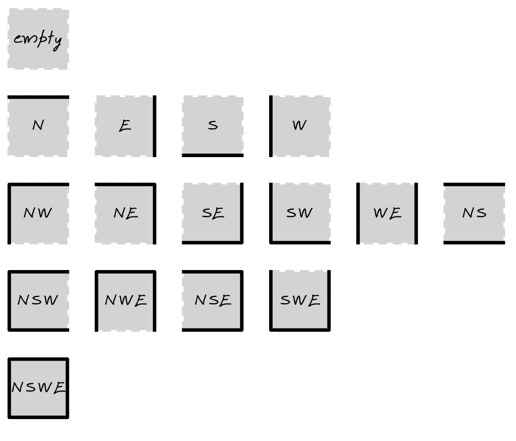
There’s one empty square, four squares with only one side, six squares with two sides, four squares with three sides, and one square with all four sides. Now, you can build almost any maze pattern with these tiles by connecting them like a jigsaw puzzle!
To compactly represent a border pattern around a square with just a single number, consider using a bit field, which maps each of the four sides to a specific binary digit. Extracting information from such a number usually requires the use of bitwise operators, which aren’t very common in Python. However, in this tutorial, you’ll use a handy shortcut from the standard library, which hides the tedious details.
Because there are four sides, you must allocate four bits that you can individually turn on or off depending on whether or not there’s a border on that side. When you convert the corresponding bit string into a decimal number, you’ll get the unambiguous representation of one of the border patterns:
| Border Sides | Bit String | Bit Count | Decimal Value |
|---|---|---|---|
| 00002 | 0 | 0 | |
| N | 00012 | 1 | 1 |
| S | 00102 | 1 | 2 |
| W | 01002 | 1 | 4 |
| E | 10002 | 1 | 8 |
| NS | 00112 | 2 | 3 |
| NW | 01012 | 2 | 5 |
| NE | 10012 | 2 | 9 |
| SW | 01102 | 2 | 6 |
| SE | 10102 | 2 | 10 |
| WE | 11002 | 2 | 12 |
| NSW | 01112 | 3 | 7 |
| NSE | 10112 | 3 | 11 |
| NWE | 11012 | 3 | 13 |
| SWE | 11102 | 3 | 14 |
| NSWE | 11112 | 4 | 15 |
As you can see, each border pattern is represented with a decimal number ranging from zero to fifteen. You can check which sides are included in the border by looking at the binary representation of the number and reading the corresponding bits. If a bit is set to one, then you’ll know that you should paint that side of the border.
The bit count, or the number of ones in the bit string, reflects the number of sides in the border. Additionally, it carries some useful information about the type of square.
For example, you can recognize a dead end by detecting precisely three sides of the border, leaving only one end to connect with other squares. Fewer than two sides may indicate a potential intersection of paths in the maze if the square isn’t a wall or part of the exterior. Specifically, a T-shaped intersection will have one side, while a four-way intersection will have none.
Detecting a corner is a bit more tricky because it requires you to compare the border against one of the four specific patterns, even though they all have exactly two sides:
- NW
- NE
- SW
- SE
This helps eliminate the other two border patterns, NS and WE, that also have two sides but aren’t corners. Their sides run in parallel instead of meeting at a corner.
Okay, now that you know what makes a square border, how do you define it in Python?
In short, you’ll use the Enum data type again, but with a slight twist. This time around, you’ll extend the enum.IntFlag base class, which is an even more specific enumeration type that implements the bit field logic. You’ll give more common names to your enum members instead of using the compass directions. Add this code to the border module:
# models/border.py

from enum import IntFlag, auto

class Border(IntFlag):
    EMPTY = 0
    TOP = auto()
    BOTTOM = auto()
    LEFT = auto()
    RIGHT = auto()
You override the default value of Border.EMPTY with a zero to indicate the absence of border sides.
This class resembles the Role enumeration that you defined in the previous section, but IntFlag allows you to do much more with its members. Rather than being a mutually exclusive choice of one member, the Border enumeration lets you combine any number of its members to create a composite value. For example, to define a closed border, you’d combine all four sides using the bitwise OR (|) operator:
>>> from maze_solver.models.border import Border

>>> border = Border.TOP | Border.BOTTOM | Border.RIGHT | Border.LEFT

>>> border
<Border.TOP|BOTTOM|LEFT|RIGHT: 15>

>>> border.name
'TOP|BOTTOM|LEFT|RIGHT'

>>> border.value
15
The .name and .value attributes of the resulting border are calculated dynamically based on the combination of its sides.
Note that the order of the individual sides doesn’t matter when you define a composite bit field:
>>> Border.TOP | Border.BOTTOM
<Border.TOP|BOTTOM: 3>

>>> Border.BOTTOM | Border.TOP
<Border.TOP|BOTTOM: 3>
Underneath, it’s a numeric value resulting from turning on the specific bits. Python will always show a consistent text representation of that value, determined by the order of your members in the class definition.
To compare your border to another border pattern, use the identity test operator (is). Alternatively, you can use the equality test operator (==) to directly compare your border against a known numeric value. Additionally, you can check if the border contains a given side using the membership test operator (in):
>>> border is Border.TOP | Border.BOTTOM | Border.RIGHT | Border.LEFT
True
>>> border is Border.TOP
False

>>> border == 15
True
>>> border == 16
False

>>> Border.TOP in border
True
Comparing an instance of enum.IntFlag to a number is possible because the flag is a subclass of the built-in integer type, just like enum.IntEnum, which you used before.
Go ahead and add a few convenience properties to your enumeration so that you can detect corners, dead ends, and intersections:
# models/border.py

from enum import IntFlag, auto

class Border(IntFlag):
    EMPTY = 0
    TOP = auto()
    BOTTOM = auto()
    LEFT = auto()
    RIGHT = auto()

    @property
    def corner(self) -> bool:
        return self in (
            self.TOP | self.LEFT,
            self.TOP | self.RIGHT,
            self.BOTTOM | self.LEFT,
            self.BOTTOM | self.RIGHT,
        )

    @property
    def dead_end(self) -> bool:
        return self.bit_count() == 3

    @property
    def intersection(self) -> bool:
        return self.bit_count() < 2
All three properties return a Boolean value. In the .corner property, you use the membership test operator (in) to check if an instance of the Border enumeration—indicated by self—is one of the predefined corners. The other two properties rely on the integer’s .bit_count() method, which returns the number of ones in the binary representation of your border.
With the Role and Border building blocks in place, you can now tie them together on a higher abstraction level. In the next section, you’ll implement the Square class.
Model the Square
The purpose of a square is to convey information about a particular location in the maze. Therefore, every square should have known coordinates that can determine its position. The square should also have a border pattern that describes the maze structure at that location. Depending on the purpose of the square, it may optionally play a special role—for example, by indicating the maze entrance.
You’ve already done the hard work by offloading most of these responsibilities to helper classes. The only remaining task is to combine them into a final square object. Open the square module and paste the following code:
# models/square.py

from dataclasses import dataclass

from maze_solver.models.border import Border
from maze_solver.models.role import Role

@dataclass(frozen=True)
class Square:
    index: int
    row: int
    column: int
    border: Border
    role: Role = Role.NONE
You’re using Python’s data class to generate the mundane code for you, which will correctly initialize instances of this class, among a few other things. Enabling the frozen parameter ensures that square objects become immutable after you create them. There’s no point in changing the values of the instance variables once they’re set.
Note: Preferring immutable objects over mutable ones where possible is considered a good programming practice, which can prevent subtle bugs caused by unexpected changes in data.
Notice that, in addition to storing the square’s row and column indices, you also keep track of its one-dimensional index within a flat sequence of squares. This way, the search algorithm can uniquely identify squares. While you could theoretically infer the index from the row and column, you’d also need to know the width and height of the maze, which are none of the square’s business. A little redundancy can sometimes keep data encapsulated.
When creating your Square instance, you must specify its index, row, column, and border pattern, but the role is completely optional. If you skip the role in the initializer, then the square will assume Role.NONE by default.
That’s it! You’ve successfully modeled the Square data type, so all the building blocks are now in place to build the maze.
Build the Maze
At the very core, a maze is an ordered collection of squares, which you can represent with a Python tuple. However, you’ll eventually want to augment your maze model with additional properties and methods, so it makes sense to wrap the sequence of squares in a custom class right away. Type the following code in your maze module:
# models/maze.py

from dataclasses import dataclass

from maze_solver.models.square import Square

@dataclass(frozen=True)
class Maze:
    squares: tuple[Square, ...]
Here, you use an immutable data class again to ensure that the underlying tuple of Square objects remains unchanged once assigned. You might be inclined to use a Python list instead of a tuple to keep your squares, but that would prevent you from caching partial results of your computations later. Python’s cache requires memoized function arguments to be hashable and, therefore, immutable.
To avoid the extra work when looping over the squares or when accessing one of them by index, you can make your class iterable and subscriptable by implementing these two special methods:
# models/maze.py

from dataclasses import dataclass
from typing import Iterator

from maze_solver.models.square import Square

@dataclass(frozen=True)
class Maze:
    squares: tuple[Square, ...]

    def __iter__(self) -> Iterator[Square]:
        return iter(self.squares)

    def __getitem__(self, index: int) -> Square:
        return self.squares[index]
The first one lets the Maze instances cooperate with the for loop, while the second one enables the square bracket notation for getting squares by index.
Next, you might want to calculate the width and height of the maze, knowing the column and row indices of the underlying squares:
# models/maze.py

from dataclasses import dataclass
from functools import cached_property
from typing import Iterator

from maze_solver.models.square import Square

@dataclass(frozen=True)
class Maze:
    squares: tuple[Square, ...]

    def __iter__(self) -> Iterator[Square]:
        return iter(self.squares)

    def __getitem__(self, index: int) -> Square:
        return self.squares[index]

    @cached_property
    def width(self):
        return max(square.column for square in self) + 1

    @cached_property
    def height(self):
        return max(square.row for square in self) + 1
You take advantage of the iterable nature of the maze by iterating over it to find the maximum column and row index of its squares with the help of the max() function. Adding 1 to the highest index accounts for the zero-based numbering of tuple indices.
Because looping is a relatively expensive operation, you cache the returned values with functools.cached_property instead of using the built-in @property decorator. As a result, the width and height are computed only once on demand, while their subsequent invocations will return the cached value.
The benefit of calculating the maze size by hand is data consistency. If you supplied the width and height through two extra parameters in the class, then there would be no guarantee that the rows and columns would match up with the flat index. On the other hand, inferring the size from the squares avoids this potential problem.
Speaking of consistency, you can also include the validation of the maze by looping over it again when it’s created to make sure that its squares have the expected rows and columns with matching indices. To do that, you’ll leverage the special method .__post_init__() to hook into the initialization process of your data class:
# models/maze.py

# ...

@dataclass(frozen=True)
class Maze:
    squares: tuple[Square, ...]

    def __post_init__(self) -> None:
        validate_indices(self)
        validate_rows_columns(self)

    # ...

def validate_indices(maze: Maze) -> None:
    assert [square.index for square in maze] == list(
        range(len(maze.squares))
    ), "Wrong square.index"

def validate_rows_columns(maze: Maze) -> None:
    for y in range(maze.height):
        for x in range(maze.width):
            square = maze[y * maze.width + x]
            assert square.row == y, "Wrong square.row"
            assert square.column == x, "Wrong square.column"
The first function checks whether the .index property of each square fits into a continuous sequence of numbers that enumerates all the squares in the maze. The second function iterates over the rows and columns in the maze, ensuring that the .row and .column attributes of the corresponding square match up with the current row and column of the loops.
Note: Watch out for the proper indentation of these functions, as they don’t belong to the class body.
Both validation functions rely on the assert statement to raise the AssertionError and prevent the maze from being created in case of invalid data.
Earlier, you stated that a maze must have an entrance and an exit, so it’s worth confirming that it has both. Go ahead and add two more validation functions:
# models/maze.py

from dataclasses import dataclass
from functools import cached_property
from typing import Iterator

from maze_solver.models.role import Role
from maze_solver.models.square import Square

@dataclass(frozen=True)
class Maze:
    squares: tuple[Square, ...]

    def __post_init__(self) -> None:
        validate_indices(self)
        validate_rows_columns(self)
        validate_entrance(self)
        validate_exit(self)

    # ...

# ...

def validate_entrance(maze: Maze) -> None:
    assert 1 == sum(
        1 for square in maze if square.role is Role.ENTRANCE
    ), "Must be exactly one entrance"

def validate_exit(maze: Maze) -> None:
    assert 1 == sum(
        1 for square in maze if square.role is Role.EXIT
    ), "Must be exactly one exit"
These count the number of squares whose role is either ENTRANCE or EXIT and verify that there’s exactly one of each. For your convenience, you might as well implement the relevant properties that’ll return the squares with those special roles:
# models/maze.py

# ...

@dataclass(frozen=True)
class Maze:
    squares: tuple[Square, ...]

    # ...

    @cached_property
    def entrance(self) -> Square:
        return next(sq for sq in self if sq.role is Role.ENTRANCE)

    @cached_property
    def exit(self) -> Square:
        return next(sq for sq in self if sq.role is Role.EXIT)

# ...
The code above calls next() on a generator expression that filters the squares by their role. Because you already validated them, you can safely assume that the appropriate squares exist in the maze, and next() won’t raise any exception.
Okay, you can finally build your first maze using the building blocks defined earlier:
>>> from maze_solver.models.border import Border
>>> from maze_solver.models.maze import Maze
>>> from maze_solver.models.role import Role
>>> from maze_solver.models.square import Square
>>> maze = Maze(
...     squares=(
...         Square(0, 0, 0, Border.TOP | Border.LEFT),
...         Square(1, 0, 1, Border.TOP | Border.RIGHT),
...         Square(2, 0, 2, Border.LEFT | Border.RIGHT, Role.EXIT),
...         Square(3, 0, 3, Border.TOP | Border.LEFT | Border.RIGHT),
...         Square(4, 1, 0, Border.BOTTOM | Border.LEFT | Border.RIGHT),
...         Square(5, 1, 1, Border.LEFT | Border.RIGHT),
...         Square(6, 1, 2, Border.BOTTOM | Border.LEFT),
...         Square(7, 1, 3, Border.RIGHT),
...         Square(8, 2, 0, Border.TOP | Border.LEFT, Role.ENTRANCE),
...         Square(9, 2, 1, Border.BOTTOM),
...         Square(10, 2, 2, Border.TOP | Border.BOTTOM),
...         Square(11, 2, 3, Border.BOTTOM | Border.RIGHT),
...     )
... )
This sample maze has twelve squares, with ten unique border patterns, arranged in three rows and four columns. The entrance to the maze is located in the bottom-left corner, while the exit is in the first row, slightly to the right. The highlighted lines indicate both special squares.
It takes a lot of imagination to visualize the final result just by looking at the code, so this is what your miniature maze will look like:

This may not be a masterpiece yet, but having a small dataset sample to work with is beneficial for several reasons. When something doesn’t work as expected, you’ll be able to spot the problem much quicker. You’ll also have a better understanding of the underlying concepts, allowing you to debug the code more effectively. Finally, because there’s little data to process, you’ll spend less time waiting for the results in your development cycle.
In this step, you identified the building blocks of the maze and implemented them in Python. Now that you can build a maze, the next step for you will be to figure out how to display the maze in a graphical form like the one depicted above.
Step 3: Visualize the Maze With Scalable Vector Graphics (SVG)
If you tried printing a crude visualization of your maze in the console using ASCII characters, then you might have noticed that it doesn’t look all that great. The reason is that, unlike squares, font glyphs are rectangular, which results in a vertically stretched image that doesn’t have the right proportions. Therefore, you need to find a different way to visualize your maze.
By the end of this step, you’ll be able to render any maze and, optionally, one of its solutions using the XML-based scalable vector graphics (SVG) format. You can use your web browser to preview the resulting SVG image, or you can open it in a vector graphics editor like Inkscape.
Model the Maze Solution
Drawing the maze can be fun on its own. However, your end goal is to solve even the most complex maze and render the shortest path from its entrance, through the corridors, to the maze exit. Finding the solution by eyeballing the maze may not always be feasible, but it should be a piece of cake for a computer program.
Add yet another module to your models package, where you’ll define a class to represent the maze solution in an object-oriented way:
maze-solver/
│
├── src/
│   │
│   └── maze_solver/
│       │
│       ├── models/
│       │   ├── __init__.py
│       │   ├── border.py
│       │   ├── maze.py
│       │   ├── role.py
│       │   ├── solution.py
│       │   └── square.py
│       │
│       └── __init__.py
│
└── pyproject.toml
The solution is a sequence of Square objects, which originates at the maze entrance and ends at the exit. Note, however, that you may jump over a few squares at a time without stepping on each as long as they line up horizontally or vertically. This reflects how you’re going to represent the path through the maze as an ordered collection of nodes in a graph.
You can implement the maze solution using the following class:
# models/solution.py

from dataclasses import dataclass

from maze_solver.models.square import Square

@dataclass(frozen=True)
class Solution:
    squares: tuple[Square, ...]
Coincidentally, this code resembles your Maze data type, which is also a data class with a .squares attribute defined as a tuple. Unlike in the maze implementation, however, this sequence is one-dimensional instead of representing rows and columns. Because of some similarities, though, you can make the Solution instances iterable and subscriptable, too, by implementing a few special methods:
# models/solution.py

from dataclasses import dataclass
from typing import Iterator

from maze_solver.models.square import Square

@dataclass(frozen=True)
class Solution:
    squares: tuple[Square, ...]

    def __iter__(self) -> Iterator[Square]:
        return iter(self.squares)

    def __getitem__(self, index: int) -> Square:
        return self.squares[index]

    def __len__(self) -> int:
        return len(self.squares)
Additionally, you add the special method .__len__() to compare the length of a solution against other possible solutions.
To make sure that instances of your Solution class represent actual solutions instead of random locations in the maze, you can add a .__post_init__() method to validate the sequence of squares:
# models/solution.py

from dataclasses import dataclass
from functools import reduce
from typing import Iterator

from maze_solver.models.role import Role
from maze_solver.models.square import Square

@dataclass(frozen=True)
class Solution:
    squares: tuple[Square, ...]

    def __post_init__(self) -> None:
        assert self.squares[0].role is Role.ENTRANCE
        assert self.squares[-1].role is Role.EXIT
        reduce(validate_corridor, self.squares)

    def __iter__(self) -> Iterator[Square]:
        return iter(self.squares)

    def __getitem__(self, index: int) -> Square:
        return self.squares[index]

    def __len__(self) -> int:
        return len(self.squares)

def validate_corridor(current: Square, following: Square) -> Square:
    assert any([
        current.row == following.row,
        current.column == following.column
    ]), "Squares must lie in the same row or column"
    return following
Validation of a solution involves checking that its first square is the maze entrance, the last square is the exit, and every two consecutive squares belong to the same row or column. You can do this by using reduce() to check that each pair of squares align either horizontally or vertically. You call any() to assert that either of the two conditions is true.
Now that you have all the building blocks of the maze and its solution, you can draw them using vector graphics.
Implement Geometric Primitives
Create a new Python package in your project with these three placeholder modules in it:
maze-solver/
│
├── src/
│   │
│   └── maze_solver/
│       │
│       ├── models/
│       │   ├── __init__.py
│       │   ├── border.py
│       │   ├── maze.py
│       │   ├── role.py
│       │   ├── solution.py
│       │   └── square.py
│       │
│       ├── view/
│       │   ├── __init__.py
│       │   ├── decomposer.py
│       │   ├── primitives.py
│       │   └── renderer.py
│       │
│       └── __init__.py
│
└── pyproject.toml
You’ll cover each of these modules in more detail in the next few sections, starting with the geometric primitives in this section. Primitives are the basic shapes—like points, lines, rectangles, or polygons—that you’ll build your maze with. Each primitive has only one responsibility, to draw itself by providing the corresponding XML representation according to SVG semantics.
To help generate SVG elements, you’re going to devise a generic function that’ll spit out an XML tag with the given name, optional value, and zero or more attributes:
# view/primitives.py

def tag(name: str, value: str | None = None, **attributes) -> str:
    attrs = "" if not attributes else " " + " ".join(
        f'{key.replace("_", "-")}="{value}"'
        for key, value in attributes.items()
    )
    if value is None:
        return f"<{name}{attrs} />"
    return f"<{name}{attrs}>{value}</{name}>"
Because SVG element attributes, such as stroke-width, can contain hyphens, which aren’t valid in Python names, you’ll automatically replace underscores (_) with hyphens (-) so that you can pass them as function arguments. If an element has no value, then you’ll use the XML self-closing tag (<element />).
Here are a few examples illustrating the use of this function:
>>> from maze_solver.view.primitives import tag

>>> # Element name
>>> tag("svg")
'<svg />'

>>> # Element name and value
>>> tag("svg", "Your web browser doesn't support SVG")
"<svg>Your web browser doesn't support SVG</svg>"

>>> # Element name and attributes (including one with a hyphen)
>>> tag("svg", xmlns="http://www.w3.org/2000/svg", stroke_linejoin="round")
'<svg xmlns="http://www.w3.org/2000/svg" stroke-linejoin="round" />'

>>> # Element name, value, and attributes
>>> tag("svg", "SVG not supported", width="100%", height="100%")
'<svg width="100%" height="100%">SVG not supported</svg>'

>>> # Nested elements
>>> tag("svg", tag("rect", fill="blue"), width="100%")
'<svg width="100%"><rect fill="blue" /></svg>'
The element name is the first and only required parameter of the function. The second parameter is the optional value. Notice that both are positional arguments, while element attributes are variable-length keyword arguments. You can also nest elements by using the output of one call to the function as input for another.
To take advantage of static duck typing, which your type checker tool can leverage, you’ll define a protocol or an interface common to all geometric primitives:
# view/primitives.py

from typing import Protocol

class Primitive(Protocol):
    def draw(self, **attributes) -> str:
        ...

# ...
Because protocols are about the interface rather than implementation, it’s common to find either the pass statement or the ellipsis literal (...) in their method bodies. Both work as a placeholder to silence the Python interpreter, which requires that every block of code starting with a colon must not be empty.
The type checker will consider any class implementing the .draw() method with this signature as a subtype of Primitive, even if they’re unrelated through inheritance. The most basic primitive is a Euclidean point comprising the x and y coordinates:
# view/primitives.py

from typing import NamedTuple, Protocol

class Primitive(Protocol):
    def draw(self, **attributes) -> str:
        ...

class Point(NamedTuple):
    x: int
    y: int

    def draw(self, **attributes) -> str:
        return f"{self.x},{self.y}"

    def translate(self, x=0, y=0) -> "Point":
        return Point(self.x + x, self.y + y)

# ...
The class extends a named tuple but not your Primitive protocol. It’s sufficient that it implements the .draw() method, which returns an SVG point as a Python string, to define a concrete primitive. Later, you’ll need to translate your points in x and y directions, so you also implement a relevant method. Because named tuples are immutable, translating a point creates a brand-new object.
The next most basic primitive is a line segment delimited by starting and ending points:
# view/primitives.py

# ...

class Line(NamedTuple):
    start: Point
    end: Point

    def draw(self, **attributes) -> str:
        return tag(
            "line",
            x1=self.start.x,
            y1=self.start.y,
            x2=self.end.x,
            y2=self.end.y,
            **attributes,
        )

# ...
This time, the .draw() method returns an SVG line, which is a stand-alone element rather than a value of an attribute.
Two other primitives closely related to a line are SVG polylines and polygons, which extend the idea of a line:
# view/primitives.py

# ...

class Polyline(tuple[Point, ...]):
    def draw(self, **attributes) -> str:
        points = " ".join(point.draw() for point in self)
        return tag("polyline", points=points, **attributes)

class Polygon(tuple[Point, ...]):
    def draw(self, **attributes) -> str:
        points = " ".join(point.draw() for point in self)
        return tag("polygon", points=points, **attributes)

# ...
They’re both tuples of two or more points, which look nearly identical. The difference is that a polygon is closed, meaning it connects the first and last point, while the polyline isn’t, leaving the last point unconnected.
Note: In case you were wondering, the points parameter must be passed as a keyword argument to avoid conflating it with the value positional argument.
Sometimes, it may be more convenient to combine existing lines instead of individual points, especially when they don’t form a continuous polyline. That’s when a DisjointLines primitive comes in handy:
# view/primitives.py

# ...

class DisjointLines(tuple[Line, ...]):
    def draw(self, **attributes) -> str:
        return "".join(line.draw(**attributes) for line in self)

# ...
Note that this is merely a logical collection of lines and has no SVG equivalent. Other, more specific SVG primitives that you’ll be interested in include a rectangle and a text element:
# view/primitives.py

from dataclasses import dataclass
from typing import NamedTuple, Protocol

# ...

@dataclass(frozen=True)
class Rect:
    top_left: Point | None = None

    def draw(self, **attributes) -> str:
        if self.top_left:
            attrs = attributes | {"x": self.top_left.x, "y": self.top_left.y}
        else:
            attrs = attributes
        return tag("rect", **attrs)

@dataclass(frozen=True)
class Text:
    content: str
    point: Point

    def draw(self, **attributes) -> str:
        return tag(
            "text",
            self.content,
            x=self.point.x,
            y=self.point.y,
            **attributes
        )

# ...
You implement them as data classes rather than tuples or named tuples because they’re not inherently sequences of elements. The rectangle accepts an optional top-left corner, whose coordinates get mixed in with the rest of the attributes through the union operator (|).
Last but not least, you’ll apply the null object pattern again by implementing a dummy NullPrimitive, which returns an empty string:
# view/primitives.py

# ...

class NullPrimitive:
    def draw(self, **attributes) -> str:
        return ""

# ...
It’ll let you avoid checking for a special case when there are no primitives to represent something in SVG, ultimately leading to cleaner and more readable code.
Next up, you’ll put your primitives to use by decomposing various border patterns around the maze’s squares into SVG elements.
Decompose a Border Into Primitives
Open your decomposer module and type the following function stub at the top of the file, which you’ll continue editing in this section:
# view/decomposer.py

from maze_solver.models.border import Border
from maze_solver.view.primitives import (
    Line,
    Point,
    Primitive,
)

def decompose(border: Border, top_left: Point, square_size: int) -> Primitive:
    top_right: Point = top_left.translate(x=square_size)
    bottom_right: Point = top_left.translate(x=square_size, y=square_size)
    bottom_left: Point = top_left.translate(y=square_size)

    top = Line(top_left, top_right)
    bottom = Line(bottom_left, bottom_right)
    left = Line(top_left, bottom_left)
    right = Line(top_right, bottom_right)
The function takes a border pattern, the top-left corner of the corresponding square in SVG coordinates, and the desired square size in SVG coordinates as input. Its goal is to decompose the border into a relevant geometric primitive that you can draw.
First, you locate the other corners of the current square’s border by translating the point that was provided to you as a function parameter. Next, you create the four sides of the border by connecting the corners into lines accordingly. Once you have all the sides and corners, you can construct the polygon, polyline, or lines associated with the given border pattern.
As you may remember, there are sixteen unique patterns, which your function needs to recognize and map to the correct primitives.
There’s only one pattern consisting of all four sides, which you can turn into a polygon:
# view/decomposer.py

from maze_solver.models.border import Border
from maze_solver.view.primitives import (
    Line,
    Point,
    Polygon,
    Primitive,
)

def decompose(border: Border, top_left: Point, square_size: int) -> Primitive:
    top_right: Point = top_left.translate(x=square_size)
    bottom_right: Point = top_left.translate(x=square_size, y=square_size)
    bottom_left: Point = top_left.translate(y=square_size)

    top = Line(top_left, top_right)
    bottom = Line(bottom_left, bottom_right)
    left = Line(top_left, bottom_left)
    right = Line(top_right, bottom_right)

    if border is Border.LEFT | Border.TOP | Border.RIGHT | Border.BOTTOM:
        return Polygon(
            [
                top_left,
                top_right,
                bottom_right,
                bottom_left,
            ]
        )
You compare the square’s border to a predefined pattern to determine whether they match. Next, there are four possible patterns with three sides, which you can describe by the bottom-left-top, left-top-right, top-right-bottom, and right-bottom-left directions:
# view/decomposer.py

from maze_solver.models.border import Border
from maze_solver.view.primitives import (
    Line,
    Point,
    Polygon,
    Polyline,
    Primitive,
)

def decompose(border: Border, top_left: Point, square_size: int) -> Primitive:
    # ...

    if border is Border.BOTTOM | Border.LEFT | Border.TOP:
        return Polyline(
            [
                bottom_right,
                bottom_left,
                top_left,
                top_right,
            ]
        )

    if border is Border.LEFT | Border.TOP | Border.RIGHT:
        return Polyline(
            [
                bottom_left,
                top_left,
                top_right,
                bottom_right,
            ]
        )

    if border is Border.TOP | Border.RIGHT | Border.BOTTOM:
        return Polyline(
            [
                top_left,
                top_right,
                bottom_right,
                bottom_left,
            ]
        )

    if border is Border.RIGHT | Border.BOTTOM | Border.LEFT:
        return Polyline(
            [
                top_right,
                bottom_right,
                bottom_left,
                top_left,
            ]
        )
You return a polyline, leaving one missing side in each case. Then, there are six border patterns with two sides, including four patterns—left-top, top-right, bottom-left, and right-bottom—which also form a polyline:
# view/decomposer.py

# ...

def decompose(border: Border, top_left: Point, square_size: int) -> Primitive:
    # ...

    if border is Border.LEFT | Border.TOP:
        return Polyline(
            [
                bottom_left,
                top_left,
                top_right,
            ]
        )

    if border is Border.TOP | Border.RIGHT:
        return Polyline(
            [
                top_left,
                top_right,
                bottom_right,
            ]
        )

    if border is Border.BOTTOM | Border.LEFT:
        return Polyline(
            [
                bottom_right,
                bottom_left,
                top_left,
            ]
        )

    if border is Border.RIGHT | Border.BOTTOM:
        return Polyline(
            [
                top_right,
                bottom_right,
                bottom_left,
            ]
        )
The two remaining two-sided patterns, left-right and top-bottom, must be represented as two disjoint lines, which run in parallel:
# view/decomposer.py

from maze_solver.models.border import Border
from maze_solver.view.primitives import (
    DisjointLines,
    Line,
    Point,
    Polygon,
    Polyline
    Primitive,
)

def decompose(border: Border, top_left: Point, square_size: int) -> Primitive:
    # ...

    if border is Border.LEFT | Border.RIGHT:
        return DisjointLines([left, right])

    if border is Border.TOP | Border.BOTTOM:
        return DisjointLines([top, bottom])
Next, you have four patterns with only one side for each compass direction:
# view/decomposer.py

# ...

def decompose(border: Border, top_left: Point, square_size: int) -> Primitive:
    # ...

    if border is Border.TOP:
        return top

    if border is Border.RIGHT:
        return right

    if border is Border.BOTTOM:
        return bottom

    if border is Border.LEFT:
        return left
Notice that you return the lines you created at the very beginning of the function. Finally, there’s the only case of an empty border pattern without any visual representation, which you can map to the null object primitive:
# view/decomposer.py

from maze_solver.models.border import Border
from maze_solver.view.primitives import (
    DisjointLines,
    Line,
    NullPrimitive,
    Point,
    Polygon,
    Polyline
    Primitive,
)

def decompose(border: Border, top_left: Point, square_size: int) -> Primitive:
    # ...

    return NullPrimitive()
Whew, that was a lot to take in! Now that the hard work is done, you can put the pieces together to achieve some tangible results. It’s time to build the scalable vector graphics renderer.
Build the SVG Renderer
Your scalable vector graphics renderer will take the square size and line width in pixel coordinates as input parameters. At the same time, it’ll assume sensible defaults so that you don’t have to fiddle with numbers to get started:
# view/renderer.py

from dataclasses import dataclass

@dataclass(frozen=True)
class SVGRenderer:
    square_size: int = 100
    line_width: int = 6

    @property
    def offset(self):
        return self.line_width // 2
The offset is the distance from the top and left edge of the drawing space, which takes your line width into account. Without it, a line starting at the top-left corner would be drawn at the very edge of the canvas and partially out of view.
The renderer returns a lightweight SVG object, which wraps the textual XML content:
# view/renderer.py

from dataclasses import dataclass

from maze_solver.models.maze import Maze
from maze_solver.models.solution import Solution

@dataclass(frozen=True)
class SVG:
    xml_content: str

@dataclass(frozen=True)
class SVGRenderer:
    square_size: int = 100
    line_width: int = 6

    @property
    def offset(self):
        return self.line_width // 2

    def render(self, maze: Maze, solution: Solution | None = None) -> SVG:
        ...
Later, you’ll add code in the SVG wrapper class to allow for viewing the rendered maze in your web browser. Rendering an SVG image boils down to decomposing the maze and its optional solution into geometric primitives, which you turn into XML tags mashed together into a string:
# view/renderer.py

from dataclasses import dataclass

from maze_solver.models.maze import Maze
from maze_solver.models.solution import Solution
from maze_solver.view.primitives import tag

@dataclass(frozen=True)
class SVG:
    xml_content: str

@dataclass(frozen=True)
class SVGRenderer:
    square_size: int = 100
    line_width: int = 6

    @property
    def offset(self):
        return self.line_width // 2

    def render(self, maze: Maze, solution: Solution | None = None) -> SVG:
        margins = 2 * (self.offset + self.line_width)
        width = margins + maze.width * self.square_size
        height = margins + maze.height * self.square_size
        return SVG(
            tag(
                "svg",
                self._get_body(maze, solution),
                xmlns="http://www.w3.org/2000/svg",
                stroke_linejoin="round",
                width=width,
                height=height,
                viewBox=f"0 0 {width} {height}",
            )
        )
You calculate the SVG dimensions based on the size of your maze and its squares, and you set the viewBox attribute accordingly. You then call a helper method to get the body of the <svg> tag, which in turn calls four other methods that you’ll implement shortly:
# view/renderer.py

# ...

@dataclass(frozen=True)
class SVGRenderer:
    # ...

    def _get_body(self, maze: Maze, solution: Solution | None) -> str:
        return "".join([
            arrow_marker(),
            background(),
            *map(self._draw_square, maze),
            self._draw_solution(solution) if solution else "",
        ])
The body of your SVG consists of a marker definition, which you’ll use to end the line representing the solution with an arrow pointing to the exit. This definition is followed by a rectangle occupying the entire view to provide a white background. Next, you render the individual squares and overlay them with the solution if supplied.
Fill the SVG Body
To get the arrow marker and the background tags, you call these two top-level functions defined at the bottom of your module:
# view/renderer.py

from dataclasses import dataclass

from maze_solver.models.maze import Maze
from maze_solver.models.solution import Solution
from maze_solver.view.primitives import Rect, tag

# ...

def arrow_marker() -> str:
    return tag(
        "defs",
        tag(
            "marker",
            tag(
                "path",
                d="M 0,0 L 10,5 L 0,10 2,5 z",
                fill="red",
                fill_opacity="50%"
            ),
            id="arrow",
            viewBox="0 0 20 20",
            refX="2",
            refY="5",
            markerUnits="strokeWidth",
            markerWidth="10",
            markerHeight="10",
            orient="auto"
        )
    )

def background() -> str:
    return Rect().draw(width="100%", height="100%", fill="white")
The <defs> and <marker> elements define an arrow shape that you’ll reference later in the SVG document. The other function uses your Rect primitive to draw a white rectangle stretched across the entire image.
Before drawing one of the maze’s squares, you need to establish where it should go by transforming its row and column into pixel coordinates:
# view/renderer.py

from dataclasses import dataclass

from maze_solver.models.maze import Maze
from maze_solver.models.solution import Solution
from maze_solver.models.square import Square
from maze_solver.view.primitives import Point, Rect, tag

# ...

@dataclass(frozen=True)
class SVGRenderer:
    # ...

    def _transform(self, square: Square, extra_offset: int = 0) -> Point:
        return Point(
            x=square.column * self.square_size,
            y=square.row * self.square_size,
        ).translate(
            x=self.offset + extra_offset,
            y=self.offset + extra_offset
        )

# ...
You scale and translate the square’s coordinates using the desired square size and offset. The resulting point is the top-left corner of your square in the SVG pixel space.
Next, you can start drawing your square, which will involve drawing a border around it, filling it with a color depending on the square type, and putting an optional label icon inside. Each of these elements will become a separate SVG tag that you’ll append to a Python list before joining together.
After transforming the coordinates, you’ll call the function that you defined in the previous section to decompose a border pattern into a drawable primitive:
# view/renderer.py

from dataclasses import dataclass

from maze_solver.models.maze import Maze
from maze_solver.models.solution import Solution
from maze_solver.models.square import Square
from maze_solver.view.decomposer import decompose
from maze_solver.view.primitives import Point, Rect, tag

# ...

@dataclass(frozen=True)
class SVGRenderer:
    # ...

    def _draw_square(self, square: Square) -> str:
        top_left: Point = self._transform(square)
        tags = []
        tags.append(self._draw_border(square, top_left))
        return "".join(tags)

    def _draw_border(self, square: Square, top_left: Point) -> str:
        return decompose(square.border, top_left, self.square_size).draw(
            stroke_width=self.line_width,
            stroke="black",
            fill="none"
        )

    # ...

# ...
You draw the border around the given square in the specified pixel location by getting its geometric representation first. This is where the null object pattern shows its strength by letting you treat all border patterns in the same way, even when they don’t have any visual representation.
Note that you created a list of tags that you’ll fill with other elements associated with the same square. Apart from the border, the walls and exterior can have a background, while squares with special roles will have an extra icon inside them:
 1# view/renderer.py
 2
 3from dataclasses import dataclass
 4
 5from maze_solver.models.maze import Maze
 6from maze_solver.models.role import Role
 7from maze_solver.models.solution import Solution
 8from maze_solver.models.square import Square
 9from maze_solver.view.decomposer import decompose
10from maze_solver.view.primitives import Point, Rect, Text, tag
11
12ROLE_EMOJI = {
13    Role.ENTRANCE: "\N{pedestrian}",
14    Role.EXIT: "\N{chequered flag}",
15    Role.ENEMY: "\N{ghost}",
16    Role.REWARD: "\N{white medium star}",
17}
18
19# ...
20
21@dataclass(frozen=True)
22class SVGRenderer:
23    # ...
24
25    def _draw_square(self, square: Square) -> str:
26        top_left: Point = self._transform(square)
27        tags = []
28        if square.role is Role.EXTERIOR:
29            tags.append(exterior(top_left, self.square_size, self.line_width))
30        elif square.role is Role.WALL:
31            tags.append(wall(top_left, self.square_size, self.line_width))
32        elif emoji := ROLE_EMOJI.get(square.role):
33            tags.append(label(emoji, top_left, self.square_size // 2))
34        tags.append(self._draw_border(square, top_left))
35        return "".join(tags)
36
37    # ...
38
39# ...
40
41def exterior(top_left: Point, size: int, line_width: int) -> str:
42    return Rect(top_left).draw(
43        width=size,
44        height=size,
45        stroke_width=line_width,
46        stroke="none",
47        fill="white"
48    )
49
50def wall(top_left: Point, size: int, line_width: int) -> str:
51    return Rect(top_left).draw(
52        width=size,
53        height=size,
54        stroke_width=line_width,
55        stroke="none",
56        fill="lightgray"
57    )
58
59def label(emoji: str, top_left: Point, offset: int) -> str:
60    return Text(emoji, top_left.translate(x=offset, y=offset)).draw(
61        font_size=f"{offset}px",
62        text_anchor="middle",
63        dominant_baseline="middle"
64    )
Here’s what the highlighted lines do:
- Lines 12 to 17 define a mapping of a subset of
Rolemembers to emoji icons expressed with Unicode name aliases. - Lines 28 to 33 call one of the helper functions defined below to draw the square’s background or an icon, depending on the square’s role.
- Lines 41 to 57 define functions that draw a rectangle with either white or light gray background.
- Lines 59 to 64 define a function that draws the specified emoji icon in the middle of the square.
Finally, the last missing method in the SVGRenderer class is one that draws the solution as a line ending with an arrow marker:
# view/renderer.py

from dataclasses import dataclass

from maze_solver.models.maze import Maze
from maze_solver.models.role import Role
from maze_solver.models.solution import Solution
from maze_solver.models.square import Square
from maze_solver.view.decomposer import decompose
from maze_solver.view.primitives import Point, Polyline, Rect, Text, tag

# ...

@dataclass(frozen=True)
class SVGRenderer:
    # ...

    def _draw_solution(self, solution: Solution) -> str:
        return Polyline(
            [
                self._transform(point, self.square_size // 2)
                for point in solution
            ]
        ).draw(
            stroke_width=self.line_width * 2,
            stroke_opacity="50%",
            stroke="red",
            fill="none",
            marker_end="url(#arrow)"
        )

    # ...

# ...
You transform the squares of the solution to get their corresponding pixel coordinates. Notice that you add an extra offset to center the solution’s line vertically and horizontally in each square. The marker-end SVG attribute refers to the SVG object identified as #arrow, which you defined earlier.
At this point, you can print the resulting SVG in the console or save its XML content to a local file:
>>> from pathlib import Path

>>> from maze_solver.models.border import Border
>>> from maze_solver.models.maze import Maze
>>> from maze_solver.models.role import Role
>>> from maze_solver.models.solution import Solution
>>> from maze_solver.models.square import Square
>>> from maze_solver.view.renderer import SVGRenderer

>>> maze = Maze(
...     squares=(
...         Square(0, 0, 0, Border.TOP | Border.LEFT),
...         Square(1, 0, 1, Border.TOP | Border.RIGHT),
...         Square(2, 0, 2, Border.LEFT | Border.RIGHT, Role.EXIT),
...         Square(3, 0, 3, Border.TOP | Border.LEFT | Border.RIGHT),
...         Square(4, 1, 0, Border.BOTTOM | Border.LEFT | Border.RIGHT),
...         Square(5, 1, 1, Border.LEFT | Border.RIGHT),
...         Square(6, 1, 2, Border.BOTTOM | Border.LEFT),
...         Square(7, 1, 3, Border.RIGHT),
...         Square(8, 2, 0, Border.TOP | Border.LEFT, Role.ENTRANCE),
...         Square(9, 2, 1, Border.BOTTOM),
...         Square(10, 2, 2, Border.TOP | Border.BOTTOM),
...         Square(11, 2, 3, Border.BOTTOM | Border.RIGHT),
...     )
... )

>>> solution = Solution(squares=tuple(maze[i] for i in (8, 11, 7, 6, 2)))
>>> svg = SVGRenderer().render(maze, solution)

>>> with Path("maze.svg").open(mode="w", encoding="utf-8") as file:
...     file.write(svg.xml_content)
...
This will save the rendered maze and your manually built solution in a file named maze.svg, which you can open using an external editor or viewer. However, it would be much more convenient to have a .preview() method on the SVG instance that you could call directly to have the image displayed to you. You’ll implement that method now.
Preview the Rendered Maze and Its Solution
These days, modern web browsers support scalable vector graphics out of the box, making them ideal SVG viewers. Websites embed SVG elements within their HTML content, style them using CSS, and even animate and interact with them dynamically through JavaScript. You’ll leverage some of these features to show your rendered SVG image using Python.
Head over to the renderer module again and add an .html_content property in your SVG class:
# view/renderer.py

import textwrap
from dataclasses import dataclass

from maze_solver.models.maze import Maze
from maze_solver.models.role import Role
from maze_solver.models.solution import Solution
from maze_solver.models.square import Square
from maze_solver.view.decomposer import decompose
from maze_solver.view.primitives import Point, Polyline, Rect, Text, tag

# ...

@dataclass(frozen=True)
class SVG:
    xml_content: str

    @property
    def html_content(self) -> str:
        return textwrap.dedent("""\
        <!DOCTYPE html>
        <html lang="en">
        <head>
          <meta charset="utf-8">
          <meta name="viewport" content="width=device-width, initial-scale=1">
          <title>SVG Preview</title>
        </head>
        <body>
        {0}
        </body>
        </html>""").format(self.xml_content)

# ...
This property returns a minimal HTML5 website with your rendered SVG image in its body. You use textwrap.dedent() to remove the leading whitespace from each line of your HTML template and replace the {0} placeholder with the object’s .xml_content attribute. Note that, in this case, using the str.format() method is preferable over an f-string literal, which would affect the indentation of the lines in an undesirable way.
This is what the output will look like when you print it against a sample SVG instance:
>>> from maze_solver.view.renderer import SVG
>>> svg = SVG('<svg><rect width="30" height="20" fill="red" /></svg>')
>>> print(svg.html_content)
<!DOCTYPE html>
<html lang="en">
<head>
  <meta charset="utf-8">
  <meta name="viewport" content="width=device-width, initial-scale=1">
  <title>SVG Preview</title>
</head>
<body>
<svg><rect width="30" height="20" fill="red" /></svg>
</body>
</html>
If you save this piece of HTML in a file and open it with your web browser, then you’ll see a small red rectangle in the top-left corner. However, you can automate these steps using a few modules in Python’s standard library.
Define the .preview() method in your class, which will save the HTML to a temporary file and open it using your web browser:
# view/renderer.py

import tempfile
import textwrap
import webbrowser
from dataclasses import dataclass

from maze_solver.models.maze import Maze
from maze_solver.models.role import Role
from maze_solver.models.solution import Solution
from maze_solver.models.square import Square
from maze_solver.view.decomposer import decompose
from maze_solver.view.primitives import Point, Polyline, Rect, Text, tag

# ...

@dataclass(frozen=True)
class SVG:
    xml_content: str

    @property
    def html_content(self) -> str:
        return textwrap.dedent("""\
        <!DOCTYPE html>
        <html lang="en">
        <head>
          <meta charset="utf-8">
          <meta name="viewport" content="width=device-width, initial-scale=1">
          <title>SVG Preview</title>
        </head>
        <body>
        {0}
        </body>
        </html>""").format(self.xml_content)

    def preview(self) -> None:
        with tempfile.NamedTemporaryFile(
            mode="w", encoding="utf-8", suffix=".html", delete=False
        ) as file:
            file.write(self.html_content)
        webbrowser.open(f"file://{file.name}")

# ...
You create a named temporary file with the .html suffix so that your web browser can recognize it correctly. Note that you also set the delete=False flag to prevent Python from automatically deleting that file before you have a chance to load it in the first place. Next, you display the rendered SVG image in your default web browser using the webbrowser module.
Note: Make sure to put the last line of code in the .preview() method outside of the with statement’s block. Because temporary files are always buffered in the text mode, calling .write() may not immediately flush pending data onto the physical disk. Only when you manually close the file or have the with statement do it for you at the end of the block will the temporary file be written to disk.
Now, try this code snippet in your Python REPL:
>>> from maze_solver.models.border import Border
>>> from maze_solver.models.maze import Maze
>>> from maze_solver.models.role import Role
>>> from maze_solver.models.solution import Solution
>>> from maze_solver.models.square import Square
>>> from maze_solver.view.renderer import SVGRenderer

>>> maze = Maze(
...     squares=(
...         Square(0, 0, 0, Border.TOP | Border.LEFT),
...         Square(1, 0, 1, Border.TOP | Border.RIGHT),
...         Square(2, 0, 2, Border.LEFT | Border.RIGHT, Role.EXIT),
...         Square(3, 0, 3, Border.TOP | Border.LEFT | Border.RIGHT),
...         Square(4, 1, 0, Border.BOTTOM | Border.LEFT | Border.RIGHT),
...         Square(5, 1, 1, Border.LEFT | Border.RIGHT),
...         Square(6, 1, 2, Border.BOTTOM | Border.LEFT),
...         Square(7, 1, 3, Border.RIGHT),
...         Square(8, 2, 0, Border.TOP | Border.LEFT, Role.ENTRANCE),
...         Square(9, 2, 1, Border.BOTTOM),
...         Square(10, 2, 2, Border.TOP | Border.BOTTOM),
...         Square(11, 2, 3, Border.BOTTOM | Border.RIGHT),
...     )
... )

>>> solution = Solution(squares=[maze[i] for i in (8, 11, 7, 6, 2)])

>>> renderer = SVGRenderer()
>>> renderer.render(maze).preview()
>>> renderer.render(maze, solution).preview()
Isn’t it more convenient than manually writing the rendered solution each time and trying to find the resulting file with your file manager? Notice how the .preview() method lets you choose between showing the solution or not. The maze with its solution rendered in your web browser should look like this:

Having the means to quickly visualize your work is an invaluable help when you build the maze manually or when you debug a maze-solving algorithm. In the next step, you’ll add code allowing you to load a few sample mazes shipped with this tutorial.
Step 4: Load the Maze From a Binary File
At this point, you can build and draw the maze. However, creating it by hand in Python takes a lot of error-prone and tedious effort. By the end of this step, you’ll have a custom file format for the persistent storage of mazes, which you’ll be able to save and load at a push of a button. Besides that, you’ll be able to load the sample mazes supplied with this tutorial.
Design the File Format
Squares in the maze are very much like pixels in an image. One of the sample mazes included in the supporting materials has several hundred of them, but you could very easily be looking at thousands of squares in some of the larger mazes.
If you were to represent the squares as text, then they would quickly amount to a huge file size. Given that you already devised a compact representation for border patterns that leverages a bit field, it makes perfect sense to define a binary file format instead.
When defining a binary file format, the first thing you need to decide on is whether you’ll store values that can fit on a single byte or more. The reason is that different computer architectures have different endianness, which is a fancy way of saying they read a sequence of bytes in the opposite order. The two standards for the byte order are called big-endian and little-endian.
In big-endian, the most significant byte comes first, while in little-endian, the least significant byte comes first. If you wrote a numeric value using one standard but then read it with another, then you’d get an utterly garbled result, just as if you applied the wrong character encoding.
You’re going to need more than one byte to store values like the width or height of the maze, which can be far greater than the maximum byte value of 255. Because many popular file formats stick with the little-endian standard, so will you!
Binary files often begin with a fixed sequence of bytes to uniquely identify their particular format. For example, Java’s class files always start with four bytes whose hexadecimal representation reads as 0xCAFEBABE, which is one of the geeky references to coffee in the language’s vast ecosystem. Such an initial value is known as the magic number, although it can sometimes be textual.
Note: Tools like the Unix file command leverage known magic numbers to detect file types:
$ file Hello.class
Hello.class: compiled Java class data, version 62.0
In this case, the tool correctly recognized a compiled Java class file.
You can choose any magic number for your custom maze file format, but in this tutorial, you’ll use the four ASCII characters MAZE in uppercase. Their hexadecimal representation, 0x4D415A45, looks less coffee-like but is just as unique and recognizable.
Next, the magic number is usually immediately followed by a file header, which provides useful metadata about the actual data in the file. The header has a fixed structure consisting of fields, such as the width of the maze. However, the header may have a variable length—for example, due to enemy positions kept in a lookup table (LUT) or optional fields.
Note: If you envision introducing breaking changes to your file format in the future, for example, due to new features, then consider including a version field either at the beginning or before the header. This should allow you to gracefully handle slight differences across file format versions.
Each header field must have a known type, size, and offset measured in bytes since the beginning of the file so that you know where the next field begins. The maze file header will have the following three fields:
| Field | Python Type | C Type | Size in Bytes | Byte Offset |
|---|---|---|---|---|
| Format Version | int |
unsigned char |
1 | 4 |
| Maze Width | int |
unsigned int |
4 | 5 |
| Maze Height | int |
unsigned int |
4 | 9 |
The first field is a single byte with your file format version, which you may increment by one with each new release. Notice that the version field starts at an offset of four bytes because the magic number occupies the first four bytes in the file. The other two fields are unsigned integers taking up four bytes each, which means they can have values between zero and over four billion.
Once you get through the header and have complete information about the amount and layout of the data, you may start reading the file body, which is the main part of the file. It’s where you’ll find most of your data. In this case, the body will be a very long one-dimensional array of numbers representing the various border patterns around the squares and their roles.
In the next section, you’ll look into packing your file body’s data neatly on as few bytes as possible.
Choose Your Data Alignment
Although each border pattern can be defined by as little as four bits—because there are sixteen different combinations of border sides—you’ll need to use the whole byte with eight bits to represent a border. That’s because a single byte is the smallest unit of information in the digital world.
It’s the same story with your square’s role, which would require only three bits to describe the seven unique values. In total, you really only need seven bits per square to faithfully represent all possible combinations of borders and roles in your maze.
Now, it’s entirely up to you how you want to align data comprising the square’s border and role. If you don’t mind being a little wasteful, then one way would be to keep those two pieces of information as a binary word made up of two consecutive bytes. However, that would effectively allocate more than twice the storage space necessary.
A far better option is to fit both numbers, which correspond to borders and roles, on a single byte. You can do this by shifting the bits of one number a few places to the left (<<) and computing their bitwise union (|) with the other number:
>>> border = 11
>>> role = 5

>>> (role << 4) | border
91

>>> format(91, "08b")
'01011011'

>>> format(role, "b")
'101'

>>> format(border, "b")
'1011'
Here, the role number’s three bits are followed by the four bits of the border number. When you look at the resulting bit pattern from its right edge, you’ll see that the first four bits (1011) are the same as the bits of the border. The next three bits (101) to the left come from the role. Finally, the most significant bit remains unused, so its value will always be zero.
Despite using plain integers in this demonstration example, you’ll get an identical result when you replace them with your Border and Role enumeration members:
>>> from maze_solver.models.square import Border
>>> from maze_solver.models.square import Role

>>> border = Border.TOP | Border.BOTTOM | Border.RIGHT
>>> role = Role.REWARD

>>> border
<Border.TOP|BOTTOM|RIGHT: 11>

>>> role
<Role.REWARD: 5>

>>> (role << 4) | border.value
91
One crucial difference, though, is that you have to explicitly refer to the .value attribute of the border or cast the border to int(). Otherwise, Python would interpret the highlighted line of code as an attempt to make a compound Border member instead of an integer number. The underlying enum.IntFlag data type overwrites the bitwise OR (|) operator to mean something other than its usual definition.
The combined border and role is your square value, which you’ll keep in the array of numbers in the file body. You can decipher the border by superimposing a bitmask on top of the square value to isolate specific bits. To get the role back, you’ll use the bitwise right-shift operator (>>), which brings the bits shifted earlier to their original position:
>>> square_value = 91

>>> border = square_value & 0b1111
>>> role = square_value >> 4

>>> border
11

>>> role
5
In this case, the bitmask 0b1111 lets you extract the four least significant bits from a number while disregarding bits to the left. Note that you can express the same bitmask in different numeral systems. It’s customary to use the hexadecimal system because it’s usually the most compact. For example, 0b1111 is the binary counterpart of 15 in the decimal system and the equivalent 0xf in the hexadecimal system.
Finally, you can pass the extracted numeric values to the relevant class constructors of your enumeration types:
>>> from maze_solver.models.square import Border
>>> from maze_solver.models.square import Role

>>> square_value = 91

>>> Border(square_value & 0xf)
<Border.TOP|BOTTOM|RIGHT: 11>

>>> Role(square_value >> 4)
<Role.REWARD: 5>
Congratulations! You’ve just defined a custom binary file format that’ll allow you to share your wonderful mazes with friends or keep them on disk to yourself. Note that this isn’t the only way to organize data in binary files. Some applications have specific needs, which may require the ability to quickly append data at the end of the file without rewriting its header. In such a case, you’d store data in blocks pointing to one another.
As you can see, there’s a lot to consider when designing a custom binary file format. Fortunately, having all that behind you now, it’s time to start digging into the implementation.
Prepare the Placeholder Modules
As before, you’re going to make some space for your code. Go ahead and create another Python package with these two placeholder modules in it:
maze-solver/
│
├── src/
│   │
│   └── maze_solver/
│       │
│       ├── models/
│       │   ├── __init__.py
│       │   ├── border.py
│       │   ├── maze.py
│       │   ├── role.py
│       │   ├── solution.py
│       │   └── square.py
│       │
│       ├── persistence/
│       │   ├── __init__.py
│       │   ├── file_format.py
│       │   └── serializer.py
│       │
│       ├── view/
│       │   ├── __init__.py
│       │   ├── decomposer.py
│       │   ├── primitives.py
│       │   └── renderer.py
│       │
│       └── __init__.py
│
└── pyproject.toml
The file_format module will contain your file header and its body, while the serializer module will provide the loading and saving routines.
Next up, you’ll define a Python class to represent your file header.
Define the File Header
Remember that the header follows the magic number, which uniquely identifies your file format. To avoid hard-coding literal numeric values, it makes sense to keep your magic number in a Python constant, which you can refer to by name.
Note: Interestingly enough, using unnamed numeric literals, such as 3.1415 to mean π, is known as the magic number anti-pattern. So, the term can take either a positive or negative meaning, depending on the context.
You can define the magic number as a read-only bytes object in Python by prepending the letter b to a string literal:
# persistence/file_format.py

MAGIC_NUMBER: bytes = b"MAZE"
Even though a bytes literal looks similar to a Python string, it’s actually a disguised sequence of integers in the range of 0 and 255. The letters M, A, Z, and E get internally turned into their ASCII codes:
>>> list(b"MAZE")
[77, 65, 90, 69]

>>> b"\x4D\x41\x5A\x45"
b'MAZE'
Because you can only use ASCII characters in such a literal, it may sometimes be more convenient to encode them with the hexadecimal notation (\x) as an alternative. In general, dealing with bytes instead of characters is preferable when you work with binary data.
The file header is perhaps best modeled as a Python data class, letting you declare the fields and their types in the expected order:
# persistence/file_format.py

from dataclasses import dataclass

MAGIC_NUMBER: bytes = b"MAZE"

@dataclass(frozen=True)
class FileHeader:
    format_version: int
    width: int
    height: int
This definition closely follows the table that you saw at the beginning of the current step in the tutorial. There are three mandatory fields in the header, all represented as integers in Python.
A file header object should be capable of writing its own content into a supplied binary file. You can use the standard library’s struct module to tell Python how to serialize the individual fields as C data types:
# persistence/file_format.py

import struct
from dataclasses import dataclass
from typing import BinaryIO

MAGIC_NUMBER: bytes = b"MAZE"

@dataclass(frozen=True)
class FileHeader:
    format_version: int
    width: int
    height: int

    def write(self, file: BinaryIO) -> None:
        file.write(MAGIC_NUMBER)
        file.write(struct.pack("B", self.format_version))
        file.write(struct.pack("<2I", self.width, self.height))
You start by dumping the bytes of your magic number and then proceed to write the remaining fields using types encoded with a special format string. The uppercase letter B stands for unsigned byte, which agrees with your expected version field.
The less than symbol (<) indicates a little-endian byte order. The number that follows communicates how many consecutive values of the same type you’re going to provide. Finally, the uppercase letter I denotes a 32-bit unsigned integer type.
So, the string <2I means two unsigned integers, one after the other, in little-endian order. It makes sense to group as many fields together as possible to limit the number of expensive system calls that write a block of data to the file.
Reading back the header from a file is fairly similar to writing it, only in reverse order:
 1# persistence/file_format.py
 2
 3import struct
 4from dataclasses import dataclass
 5from typing import BinaryIO
 6
 7MAGIC_NUMBER: bytes = b"MAZE"
 8
 9@dataclass(frozen=True)
10class FileHeader:
11    format_version: int
12    width: int
13    height: int
14
15    @classmethod
16    def read(cls, file: BinaryIO) -> "FileHeader":
17        assert (
18            file.read(len(MAGIC_NUMBER)) == MAGIC_NUMBER
19        ), "Unknown file type"
20        format_version, = struct.unpack("B", file.read(1))
21        width, height = struct.unpack("<2I", file.read(2 * 4))
22        return cls(format_version, width, height)
23
24    def write(self, file: BinaryIO) -> None:
25        file.write(MAGIC_NUMBER)
26        file.write(struct.pack("B", self.format_version))
27        file.write(struct.pack("<2I", self.width, self.height))
At the time of reading the header from a file, no class instance exists yet, so you must define a class method that can act on the class rather than an object. Here’s a breakdown of what happens inside that method:
- Lines 17 to 19 read the number of bytes equal to the length of your magic number and compare the result with the constant. Any discrepancy will stop further processing by raising an exception to indicate an unknown file format.
- Line 20 reads a single unsigned byte and assigns the result to a local variable with the file format version. Note that there’s a comma (
,) right after the variable declaration, which is mandatory! Becausestruct.unpack()always returns a tuple, even if it only has one value, the comma helps unpack the first element from that tuple. - Line 21 reads eight bytes into two unsigned integers in the little-endian byte order. The resulting tuple is then unpacked into a matching number of local variables with the assignment operator.
- Line 22 returns a new instance of the
FileHeaderclass initialized with the local variables.
Notice that your file header is currently version-agnostic, so it should work with multiple file format versions. Sometimes, you’ll want to read only the metadata from the header despite not being able to process the file’s body due to an unsupported format.
When you finish reading the header, you’ll know how many squares there are and how they’re arranged in rows and columns. This will allow you to interpret the remaining part of the file correctly, which you’ll do now.
Define the File Body
The file body is less exciting than the header because it’s merely a stream of small integers representing border patterns and square roles in the maze. It might be your first instinct to put them in a Python list or tuple. However, the array module in the standard library provides a much better-suited data type for efficiently storing such homogeneous numeric sequences.
Lists and tuples are heterogenous, meaning you can stuff elements of all kinds into them. However, the price of that versatility is that they take up more memory and are slower to access than an array. Because you’ll be storing plain numbers instead of Python objects in the file on disk, you can take advantage of a faster and more suitable array data structure.
Your FileBody class will have only one attribute to accommodate the square values:
# persistence/file_format.py

import array
import struct
from dataclasses import dataclass
from typing import BinaryIO

MAGIC_NUMBER: bytes = b"MAZE"

# ...

@dataclass(frozen=True)
class FileBody:
    square_values: array.array
When passing an array instance to the file body object, you’ll need to ensure that the array was created with the right type code that identifies the underlying C type. In this case, you must use the uppercase letter B to mean an array of unsigned bytes. You’ll do that right before reading the file body:
# persistence/file_format.py

# ...

@dataclass(frozen=True)
class FileBody:
    square_values: array.array

    @classmethod
    def read(cls, header: FileHeader, file: BinaryIO) -> "FileBody":
        return cls(
            array.array("B", file.read(header.width * header.height))
        )
To read the body, you must’ve read the header before so that the internal file pointer is set at the right offset. Besides that, the header object is one of the parameters expected by this class method. You use the information stored in the file header to calculate the number of remaining bytes to read by multiplying the width and height of the maze. This data is then converted to a byte array and passed to the FileBody instance.
Writing the file body becomes more straightforward when you call the array’s .tobytes() method, which takes care of serializing the items into the correct data type in the requested byte order. That said, the byte order becomes irrelevant when your array contains only single-byte values:
# persistence/file_format.py

# ...

@dataclass(frozen=True)
class FileBody:
    square_values: array.array

    @classmethod
    def read(cls, header: FileHeader, file: BinaryIO) -> "FileBody":
        return cls(
            array.array("B", file.read(header.width * header.height))
        )

    def write(self, file: BinaryIO) -> None:
        file.write(self.square_values.tobytes())
Later, you’ll use the numbers stored in your array to create Border and Role instances like you did before.
Okay, you can now individually write and read the file header and body, which are the low-level details of your custom file format. However, you still need to serialize and deserialize the higher-level maze object. You’ll address that in the following sections.
Serialize the Maze
Unless you already have some data to work with, you’re better off implementing the serialization code first, which will eventually write a file that you can later use to test the loading procedure. Open the serializer module and type the following code in it:
 1# persistence/serializer.py
 2
 3import array
 4
 5from maze_solver.models.maze import Maze
 6from maze_solver.models.square import Square
 7from maze_solver.persistence.file_format import FileBody, FileHeader
 8
 9FORMAT_VERSION: int = 1
10
11def serialize(maze: Maze) -> tuple[FileHeader, FileBody]:
12    header = FileHeader(FORMAT_VERSION, maze.width, maze.height)
13    body = FileBody(array.array("B", map(compress, maze)))
14    return header, body
15
16def compress(square: Square) -> int:
17    return (square.role << 4) | square.border.value
Here’s a line-by-line explanation of what this code does:
- Lines 11 to 14 define the
serialize()function, which accepts an instance of theMazemodel that you implemented earlier. This function produces a tuple consisting of the file header and body, which you’ll later dump into a binary file. - Line 12 prepares the file header by setting a known file format version based on a constant, as there’s only one version currently supported. Other header field values are copied from the maze object that was passed as an argument.
- Line 13 populates the file body with binary values obtained by compressing the border patterns and square roles into a single byte for each square. Calling
map()on the maze instance implicitly iterates over it and applies thecompress()function on each square in the maze. - Lines 16 and 17 define a helper function, which takes a
Squareinstance as an argument and returns the correspondingRoleandBordervalues encoded as a compound bit field. It uses bitwise operators to compress the two values into a single number.
Writing the header and the body to a file is pretty straightforward, thanks to the pathlib.Path object:
# persistence/serializer.py

import array
import pathlib

from maze_solver.models.maze import Maze
from maze_solver.models.square import Square
from maze_solver.persistence.file_format import FileBody, FileHeader

FORMAT_VERSION: int = 1

def dump(maze: Maze, path: pathlib.Path) -> None:
    header, body = serialize(maze)
    with path.open(mode="wb") as file:
        header.write(file)
        body.write(file)

# ...
However, it’s important that you open the file for writing (w) in binary mode (b) to ensure that Python writes your data as is, without any implicit conversions.
With these three short functions, you can now take your miniature test maze that you built earlier and try dumping it to a file:
>>> from pathlib import Path

>>> from maze_solver.models.border import Border
>>> from maze_solver.models.maze import Maze
>>> from maze_solver.models.role import Role
>>> from maze_solver.models.square import Square
>>> from maze_solver.persistence.serializer import dump

>>> maze = Maze(
...     squares=(
...         Square(0, 0, 0, Border.TOP | Border.LEFT),
...         Square(1, 0, 1, Border.TOP | Border.RIGHT),
...         Square(2, 0, 2, Border.LEFT | Border.RIGHT, Role.EXIT),
...         Square(3, 0, 3, Border.TOP | Border.LEFT | Border.RIGHT),
...         Square(4, 1, 0, Border.BOTTOM | Border.LEFT | Border.RIGHT),
...         Square(5, 1, 1, Border.LEFT | Border.RIGHT),
...         Square(6, 1, 2, Border.BOTTOM | Border.LEFT),
...         Square(7, 1, 3, Border.RIGHT),
...         Square(8, 2, 0, Border.TOP | Border.LEFT, Role.ENTRANCE),
...         Square(9, 2, 1, Border.BOTTOM),
...         Square(10, 2, 2, Border.TOP | Border.BOTTOM),
...         Square(11, 2, 3, Border.BOTTOM | Border.RIGHT),
...     )
... )

>>> dump(maze, Path("miniature.maze"))
This should create a new file named miniature.maze in your current working directory, which is where you started the Python REPL session. If the file already exists, then it’ll get overwritten without any warning, so be careful!
To quickly verify that the file was created, head over to the file manager in your operating system and look for the new file, which should be twenty-five bytes in size. The first thirteen bytes are the header, followed by twelve bytes corresponding to the twelve squares in the maze.
If you have a hex editor or a tool like hexdump, then you can inspect the file’s binary content, which should look something like this:
$ hd miniature.maze
00000000  4d 41 5a 45 01 04 00 00  00 03 00 00 00 05 09 3c  |MAZE...........<|
00000010  0d 0e 0c 06 08 25 02 03  0a                       |.....%...|
00000019
The first column is the hexadecimal offset of the first byte in each line, which shows the next sixteen bytes of the file in a two-digit hexadecimal notation. For example, the byte at offset zero is 4d16 or 7710 in the decimal system, which corresponds to the uppercase letter M in ASCII.
Over to the right, you’ll see a text representation of the same data. The dots represent non-printable characters. Other characters depict bytes that happen to have a visual representation in ASCII.
When you discard the header, you’ll be left with the last twelve bytes of the file, which translate to the following decimal values:
>>> hex_digits = "05 09 3c 0d 0e 0c 06 08 25 02 03 0a"
>>> [int(x, 16) for x in hex_digits.split()]
[5, 9, 60, 13, 14, 12, 6, 8, 37, 2, 3, 10]
The resulting sequence of numbers consists of bit fields that should match the squares in your miniature maze. The two outliers with noticeably higher values, 60 and 37, contain extra information about the special roles of these particular squares. In their case, one must be the entrance and the other the maze’s exit.
However, you can’t know that for sure yet because you haven’t implemented the maze deserialization code. You’ll fix that now.
Deserialize the Maze
To deserialize a binary file into an instance of your Maze class, you’re going to follow the same steps but in the opposite order. Modify your serializer module by adding new functions to complement the ones that you created earlier. The first function will take a file path as an argument and return the loaded maze object:
# persistence/serializer.py

# ...

def dump(maze: Maze, path: pathlib.Path) -> None:
    header, body = serialize(maze)
    with path.open(mode="wb") as file:
        header.write(file)
        body.write(file)

def load(path: pathlib.Path) -> Maze:
    with path.open("rb") as file:
        header = FileHeader.read(file)
        if header.format_version != FORMAT_VERSION:
            raise ValueError("Unsupported file format version")
        body = FileBody.read(header, file)
        return deserialize(header, body)

# ...
You open the file for reading (r) in binary mode (b), obtain the file header, and check the file’s format version before attempting to read its body. When the file format is unsupported, you raise an exception. Otherwise, you pass the header and body to another function, which can create a new maze object based on the information provided. In the future, you can branch the code to read the file body differently depending on the detected version.
The deserializing function should look as follows:
# persistence/serializer.py

# ...

def serialize(maze: Maze) -> tuple[FileHeader, FileBody]:
    header = FileHeader(FORMAT_VERSION, maze.width, maze.height)
    body = FileBody(array.array("B", map(compress, maze)))
    return header, body

def deserialize(header: FileHeader, body: FileBody) -> Maze:
    squares: list[Square] = []
    for index, square_value in enumerate(body.square_values):
        row, column = divmod(index, header.width)
        border, role = decompress(square_value)
        squares.append(Square(index, row, column, border, role))
    return Maze(tuple(squares))

# ...
First, you create an empty list, which you then populate with Square instances by looping over the square values in the file body. To keep track of the current square index, you enumerate the values and calculate their row and column based on metadata in the header. Each bit field gets decompressed into the relevant Border and Role, which the square’s class constructor requires. Finally, you pass the squares as a tuple to the Maze constructor.
The decompression of a single square value follows the principles outlined at the beginning of this step, when you were choosing how to pack your data on a single byte:
# persistence/serializer.py

import array
import pathlib

from maze_solver.models.border import Border
from maze_solver.models.maze import Maze
from maze_solver.models.role import Role
from maze_solver.models.square import Square
from maze_solver.persistence.file_format import FileBody, FileHeader

# ...

def compress(square: Square) -> int:
    return (square.role << 4) | square.border.value

def decompress(square_value: int) -> tuple[Border, Role]:
    return Border(square_value & 0xf), Role(square_value >> 4)
The bitmask and bit shifting allow you to separate the two pieces of data from one number. Your enumerations can be seeded with those two numbers, while their resulting members can be wrapped in a tuple and returned.
Finally, you can verify whether you’ll get the same object that you started with by dumping your test maze into a file, and then loading it back:
>>> from pathlib import Path

>>> from maze_solver.models.border import Border
>>> from maze_solver.models.maze import Maze
>>> from maze_solver.models.role import Role
>>> from maze_solver.models.square import Square
>>> from maze_solver.persistence.serializer import dump, load

>>> maze = Maze(
...     squares=(
...         Square(0, 0, 0, Border.TOP | Border.LEFT),
...         Square(1, 0, 1, Border.TOP | Border.RIGHT),
...         Square(2, 0, 2, Border.LEFT | Border.RIGHT, Role.EXIT),
...         Square(3, 0, 3, Border.TOP | Border.LEFT | Border.RIGHT),
...         Square(4, 1, 0, Border.BOTTOM | Border.LEFT | Border.RIGHT),
...         Square(5, 1, 1, Border.LEFT | Border.RIGHT),
...         Square(6, 1, 2, Border.BOTTOM | Border.LEFT),
...         Square(7, 1, 3, Border.RIGHT),
...         Square(8, 2, 0, Border.TOP | Border.LEFT, Role.ENTRANCE),
...         Square(9, 2, 1, Border.BOTTOM),
...         Square(10, 2, 2, Border.TOP | Border.BOTTOM),
...         Square(11, 2, 3, Border.BOTTOM | Border.RIGHT),
...     )
... )

>>> path = Path("miniature.maze")

>>> dump(maze, path)
>>> load(path) == maze
True

>>> load(path) is maze
False
You can rely on the equality test (==) provided by your data class, which correctly compares Maze instances by their value rather than identity. While the original maze and the loaded counterpart are two distinct objects in computer memory, they compare as equal because they’re made up of the same squares!
There’s one last detail to improve in your current implementation of the maze serialization. Notice that in order to load or dump the maze to a file, you need to import both the Maze model and the relevant function from the serializer module. That’s not ideal from an object-oriented perspective, so you’ll work on that in the next section.
Add the Serializing Methods to the Maze Class
To make your Maze class more self-contained, you may augment it with .load() and .dump() methods that’ll delegate processing to their respective counterparts in the serializer module. However, doing so without any modifications would inevitably lead to the dreaded circular dependency, which Python doesn’t allow. You can’t have your class depend on functions in another module and the other way around at the same time.
There are a few ways to work around this problem, each with its pros and cons, but the most elegant solution is to break the two-way dependency in one direction if possible. Since you want to call the serializing code from within your class, removing all Maze class references from the serializer module is your only option.
Start refactoring your code by first deleting the following import statement from the serializer module:
 # persistence/serializer.py

 import array
 import pathlib

 from maze_solver.models.border import Border
-from maze_solver.models.maze import Maze
 from maze_solver.models.role import Role
 from maze_solver.models.square import Square
 from maze_solver.persistence.file_format import FileBody, FileHeader

 # ...
As soon as you do that, your code editor should flag all unresolved Maze class references in this module. You’ll find the first one in your dump() function at the top of the file. The function currently accepts a maze object as an argument, which you can replace with intermediary data transfer objects (DTOs), such as Python built-in types or other models:
 # persistence/serializer.py

 # ...

-def dump(maze: Maze, path: pathlib.Path) -> None:
+def dump_squares(
+    width: int,
+    height: int,
+    squares: tuple[Square, ...],
+    path: pathlib.Path,
+) -> None:
-    header, body = serialize(maze)
+    header, body = serialize(width, height, squares)
     with path.open(mode="wb") as file:
         header.write(file)
         body.write(file)

# ...
Rather than serializing a Maze instance, you’ll now serialize its building blocks, which the Maze class can put together again. Notice that you rename the function to convey its purpose more accurately by emphasizing its new interface.
You must also cascade this change down to the called function, serialize(), while compress() and decompress() will remain intact:
 # persistence/serializer.py

 # ...

-def serialize(maze: Maze) -> tuple[FileHeader, FileBody]:
+def serialize(
+    width: int,
+    height: int,
+    squares: tuple[Square, ...]
+) -> tuple[FileHeader, FileBody]:
-    header = FileHeader(FORMAT_VERSION, maze.width, maze.height)
+    header = FileHeader(FORMAT_VERSION, width, height)
-    body = FileBody(array.array("B", map(compress, maze)))
+    body = FileBody(array.array("B", map(compress, squares)))
     return header, body

 # ...
With this update, both dump_squares() and serialize() have compatible function signatures again.
You’ll modify your deserializing code in a similar way by getting rid of the dependency on Maze from both load() and deserialize():
 # persistence/serializer.py

 import array
 import pathlib
+from typing import Iterator

 from maze_solver.models.border import Border
 from maze_solver.models.role import Role
 from maze_solver.models.square import Square
 from maze_solver.persistence.file_format import FileBody, FileHeader

 # ...

-def load(path: pathlib.Path) -> Maze:
+def load_squares(path: pathlib.Path) -> Iterator[Square]:
    with path.open("rb") as file:
        header = FileHeader.read(file)
        if header.format_version != FORMAT_VERSION:
            raise ValueError("Unsupported file format version")
        body = FileBody.read(header, file)
        return deserialize(header, body)

-def deserialize(header: FileHeader, body: FileBody) -> Maze:
+def deserialize(header: FileHeader, body: FileBody) -> Iterator[Square]:
-    squares: list[Square] = []
     for index, square_value in enumerate(body.square_values):
         row, column = divmod(index, header.width)
         border, role = decompress(square_value)
-        squares.append(Square(index, row, column, border, role))
+        yield Square(index, row, column, border, role)
-    return Maze(tuple(squares))

# ...
The loading function is now named load_squares() to follow a consistent naming convention, and it returns an iterator of squares rather than a complete maze. Additionally, you simplified the other function, deserialize(), by turning it into a generator function, which returns a generator iterator of Square instances.
At this point, the serializer module doesn’t depend on the Maze class anymore because there are no direct references to it. You can safely update your maze model as a consequence:
# models/maze.py

from dataclasses import dataclass
from functools import cached_property
from pathlib import Path
from typing import Iterator

from maze_solver.models.role import Role
from maze_solver.models.square import Square
from maze_solver.persistence.serializer import (
    dump_squares,
    load_squares,
)

@dataclass(frozen=True)
class Maze:
    squares: tuple[Square, ...]

    @classmethod
    def load(cls, path: Path) -> "Maze":
        return Maze(tuple(load_squares(path)))

    # ...

    def dump(self, path: Path) -> None:
        dump_squares(self.width, self.height, self.squares, path)

# ...
With the class method depicted above, you can .load() squares from the specified path and turn them into a new Maze instance. Conversely, by calling .dump() on an existing maze object, you’ll dump its squares along with the necessary metadata to a given path.
Here’s an example of the Maze.load() class method in action, which loads your miniature test maze:
>>> from pathlib import Path
>>> from maze_solver.models.maze import Maze

>>> maze = Maze.load(Path("miniature.maze"))

>>> maze.width, maze.height
(4, 3)

>>> len(maze.squares)
12

>>> maze.entrance
Square(index=8,
       row=2,
       column=0,
       border=<Border.TOP|LEFT: 5>,
       role=<Role.ENTRANCE: 2>)

>>> maze.exit
Square(index=2,
       row=0,
       column=2,
       border=<Border.LEFT|RIGHT: 12>,
       role=<Role.EXIT: 3>)
Now, you only need to import one symbol from the maze_solver package to work with mazes stored in files. The deserialized object’s attribute values confirm that you successfully loaded the maze. By the way, check if you correctly guessed which squares are the entrance and exit of your miniature maze!
Why don’t you go ahead and try loading a more challenging maze from the supporting materials? For example, the labyrinth.maze has 896 squares arranged in 32 rows and 28 columns.
Free Download: Click here to download the source code and supporting materials that you’ll use to build a maze solver in Python.
You can preview it in your web browser by running the following code snippet in your Python REPL:
>>> from pathlib import Path
>>> from maze_solver.models.maze import Maze
>>> from maze_solver.view.renderer import SVGRenderer

>>> maze = Maze.load(Path("mazes") / "labyrinth.maze")
>>> len(maze.squares), maze.height, maze.width
(896, 32, 28)

>>> SVGRenderer().render(maze).preview()
Make sure that you specify the right path to the file and run this code from a virtual environment that has your maze_solver package installed. Afterward, you should see the following maze on your screen:
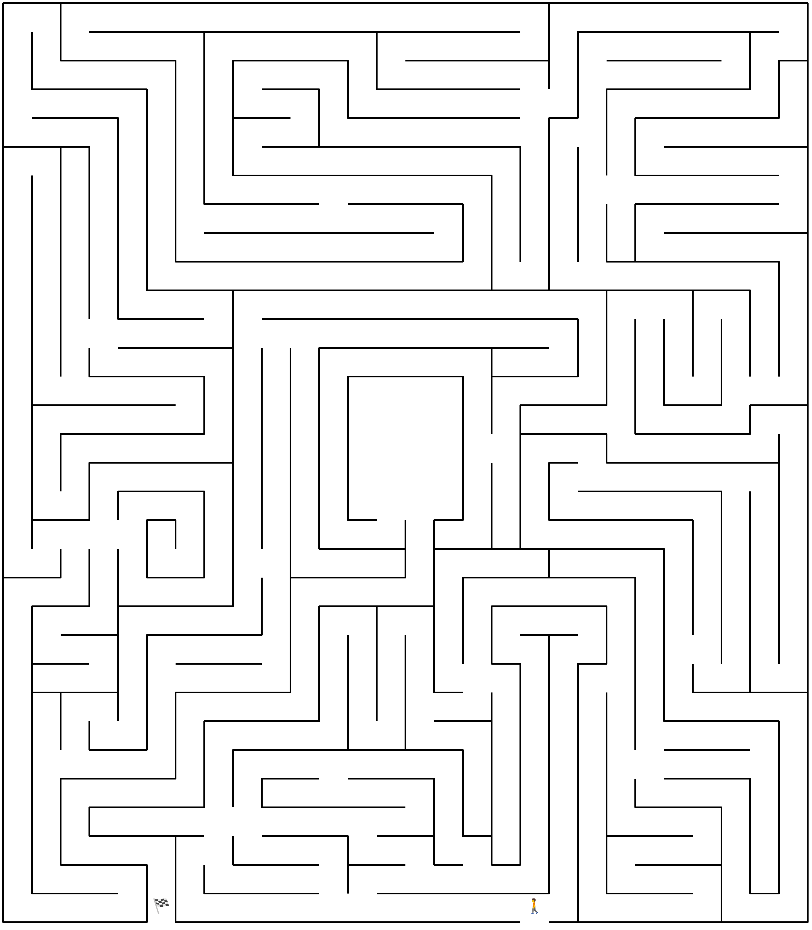
This maze was assembled from satellite and aerial photos of a real-world labyrinth in Łeba on the Baltic sea, which can take as long as forty-five minutes to complete on foot! Can you find the way out of this maze by looking at the rendered preview above? While there are no enemies, the maze is still quite tricky!
In the next and final step of this tutorial, you’ll implement a graph representation of that maze so that you can solve it with Python. In fact, you’ll be able to find the shortest path between the entrance and exit of any valid maze stored in your custom binary file format.
Step 5: Solve the Maze Using a Graph-Based Approach
At this point, you can represent the maze and its solution in an object-oriented form. You can visualize them, as well as serialize the maze using a custom binary file format. Now, it’s time to convert your maze to a graph and let Python find the shortest path from the entrance to the exit. By the end of this step, you’ll have a command-line program for solving and visualizing mazes loaded from the specified file.
Install the NetworkX Library
Graphs are an important data structure in theoretical computer science, which often come up during code interviews. While you may use them sparingly in your day-to-day programming practice, graphs can help solve a variety of problems, like finding your way out of a maze.
A graph is a set of nodes and the edges between them. Because nodes have no inherent location in space, when you convert the maze into a graph form, you lose some information about its geometry. Later, you’ll add weights to the edges to represent the cost of traversing each connection between two nodes.
Rather than reinventing the wheel, you’ll use a graph representation provided by the popular NetworkX library, which ships with a couple of useful graph algorithms. Go ahead and add this library to your pyproject.toml file now by listing it as the project’s dependency:
# pyproject.toml

[build-system]
requires = ["setuptools>=64.0.0", "wheel"]
build-backend = "setuptools.build_meta"

[project]
name = "maze-solver"
version = "1.0.0"

dependencies = [
    "networkx >= 3.0",
]
As a rule of thumb, avoid specifying concrete dependency versions directly in the pyproject.toml file, especially when you intend to use your package as a reusable library in other projects that might depend on different NetworkX versions. However, it’s always a good idea to pin dependency versions in a requirements.txt file to ensure reproducible builds.
Now, reinstall your package in the associated virtual environment using the editable mode again so that the networkx package becomes available for importing. You can also pin the specific dependencies:
(venv) $ python -m pip install -e .
(venv) $ python -m pip freeze > requirements.txt
Before moving on, you can also create another Python package in your project with the converter and solver placeholder modules:
maze-solver/
│
├── src/
│   │
│   └── maze_solver/
│       │
│       ├── graphs/
│       │   ├── __init__.py
│       │   ├── converter.py
│       │   └── solver.py
│       │
│       ├── models/
│       │   ├── __init__.py
│       │   ├── border.py
│       │   ├── maze.py
│       │   ├── role.py
│       │   ├── solution.py
│       │   └── square.py
│       │
│       ├── persistence/
│       │   ├── __init__.py
│       │   ├── file_format.py
│       │   └── serializer.py
│       │
│       ├── view/
│       │   ├── __init__.py
│       │   ├── decomposer.py
│       │   ├── primitives.py
│       │   └── renderer.py
│       │
│       └── __init__.py
│
├── pyproject.toml
└── requirements.txt
The converter module will contain a few functions for turning your maze into a graph, while the solver module will use those functions as glue code to wrap NetworkX’s algorithms and solve your maze.
Next up, you’ll start writing the converter module.
Transform the Maze Into a Graph
To create a graph, you’ll need to provide nodes and edges that connect them. You’ve already established that your maze consists of nodes that represent path intersections, dead ends, and special squares, like enemies or the entrance. However, if you connect them directly without taking the corners into account, then you won’t be able to follow the maze’s horizontal and vertical pathways:
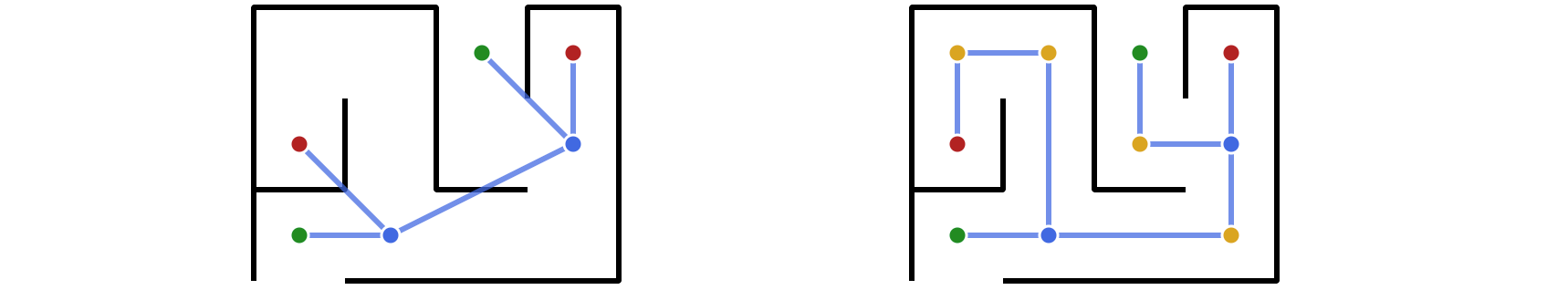
The image on the left depicts six color-coded nodes, including two intersections (blue), two dead ends (red), as well as the entrance and the exit (green). The image on the right is almost the same, but it has four additional corners (yellow), which help you preserve the maze’s layout.
Your Border model can already identify a .corner, .intersection, and .dead_end, while the Role model will tell you whether the associated square has some special function in the maze. You can treat the square as a synonym for a graph node because the NetworkX library lets you use any object as a node—as long as it’s hashable. The Square class is hashable out of the box because you implemented it as an immutable, or frozen, data class.
Note: The reason why graph nodes must be hashable is that NetworkX maintains an internal adjacency matrix of the nodes, which are kept as keys in a Python dictionary.
To use consistent terminology, you’ll define a type alias for the Square class so that you can refer to it as a Node in your code. Once you’ve done this, you’ll model the edge as a pair of two nodes, which you can implement as a named tuple:
# graphs/converter.py

from typing import NamedTuple, TypeAlias

from maze_solver.models.square import Square

Node: TypeAlias = Square

class Edge(NamedTuple):
    node1: Node
    node2: Node
It’s possible to represent edges of directed graphs with this class because it’s an ordered pair. But you’ll only consider undirected graphs with two-way connections between their nodes for now.
Now that you have a representation for nodes and edges, you can start transforming your maze into a graph by first getting a collection of nodes from it. The simple way would be to turn all squares into nodes. However, capturing only intersections, corners, and dead ends as nodes can lead to a more efficient and accurate solution for solving mazes. You can identify these nodes by checking the role and border pattern of each square in the maze:
# graphs/converter.py

from typing import NamedTuple, TypeAlias

from maze_solver.models.maze import Maze
from maze_solver.models.role import Role
from maze_solver.models.square import Square

Node: TypeAlias = Square

class Edge(NamedTuple):
    node1: Node
    node2: Node

def get_nodes(maze: Maze) -> set[Node]:
    nodes: set[Node] = set()
    for square in maze:
        if square.role in (Role.EXTERIOR, Role.WALL):
            continue
        if square.role is not Role.NONE:
            nodes.add(square)
        if (
            square.border.intersection
            or square.border.dead_end
            or square.border.corner
        ):
            nodes.add(square)
    return nodes
If a square is marked as either a wall or exterior, then it’s definitely not part of the graph, so you skip it with the continue statement. Otherwise, if the square has some special role other than None, then you record it as a graph node. Finally, regardless of the square’s role, you take note of intersections, dead ends, and corners.
Note: Thanks to using a Python set, you don’t have to worry about adding the same square more than once when, for example, a reward happens to be placed at an intersection. That’s because sets filter out duplicates.
Next, you’ll need to connect your nodes with edges. To do that, you’ll take advantage of the fact that the maze is a rectangular grid. That means you can loop through the nodes that you just identified, checking to the right and down for any adjacent nodes in the maze and stopping once you reach a wall:
# graphs/converter.py

from typing import NamedTuple, TypeAlias

from maze_solver.models.border import Border
from maze_solver.models.maze import Maze
from maze_solver.models.role import Role
from maze_solver.models.square import Square

# ...

def get_edges(maze: Maze, nodes: set[Node]) -> set[Edge]:
    edges: set[Edge] = set()
    for source_node in nodes:
        # Follow right:
        node = source_node
        for x in range(node.column + 1, maze.width):
            if node.border & Border.RIGHT:
                break
            node = maze.squares[node.row * maze.width + x]
            if node in nodes:
                edges.add(Edge(source_node, node))
                break
        # Follow down:
        node = source_node
        for y in range(node.row + 1, maze.height):
            if node.border & Border.BOTTOM:
                break
            node = maze.squares[y * maze.width + node.column]
            if node in nodes:
                edges.add(Edge(source_node, node))
                break
    return edges
You look for the immediate neighbors of each node supplied to the function. In this case, you move east and south in the maze, but you could just as well follow the opposite directions, remembering to change the loop indexing and wall detection accordingly. You use the bitwise AND operator (&) to check if a border around the current square has either the right or bottom side, indicating a wall that terminates the search in that direction.
On the other hand, if you find that a square located in the same row or column as your source node is also present in the set of nodes, and there’s no wall between them, then you create an Edge instance. Knowing the edges is sufficient to define a new NetworkX graph object:
# graphs/converter.py

from typing import NamedTuple, TypeAlias

import networkx as nx

from maze_solver.models.border import Border
from maze_solver.models.maze import Maze
from maze_solver.models.role import Role
from maze_solver.models.square import Square

Node: TypeAlias = Square

class Edge(NamedTuple):
    node1: Node
    node2: Node

def make_graph(maze: Maze) -> nx.Graph:
    return nx.Graph(get_edges(maze, get_nodes(maze)))

# ...
The initializer method of nx.Graph can optionally take various graph data types, including a collection of edges. Normally, you should create an instance of nx.MultiGraph to account for parallel edges that might appear in one of your mazes. However, the extra corners that you’ve added before make each parallel connection unique, so there’s no need to use a multigraph in this case.
In the next section, you’ll use NetworkX to find the shortest path from the entrance to the exit of the maze.
Find the Shortest Path
Open the solver module and define the following function, which takes a Maze instance and returns the corresponding Solution:
# graphs/solver.py

import networkx as nx

from maze_solver.graphs.converter import make_graph
from maze_solver.models.maze import Maze
from maze_solver.models.solution import Solution

def solve(maze: Maze) -> Solution | None:
    try:
        return Solution(
            squares=tuple(
                nx.shortest_path(
                    make_graph(maze),
                    source=maze.entrance,
                    target=maze.exit,
                )
            )
        )
    except nx.NetworkXException:
        return None
In this function, you call your make_graph() function from the converter module to obtain an nx.Graph object, which you then pass to the nx.shortest_path() function. Notice how the maze’s .entrance and .exit properties help you specify the source and target nodes in the graph. In case NetworkX can’t find the shortest path between them, you handle the exception and return None to indicate that there’s no solution.
That’s all you need to solve the maze with NetworkX! You can now test this pathfinding algorithm on your pocket-size maze:
>>> from pathlib import Path
>>> from maze_solver.graphs.solver import solve
>>> from maze_solver.models.maze import Maze
>>> from maze_solver.view.renderer import SVGRenderer

>>> maze = Maze.load(Path("mazes") / "miniature.maze")
>>> solution = solve(maze)

>>> len(solution)
6

>>> [square.index for square in solution]
[8, 9, 11, 7, 6, 2]

>>> SVGRenderer().render(maze, solution).preview()
The solution has six nodes, starting at a square with index eight and ending at a square with index two. When you render the solution, you’ll see the following image in your web browser:

Okay. That was a fairly simple maze, but what about that giant labyrinth composed of hundreds of squares you saw before? Well, you can check it out for yourself by changing the filename to labyrinth.maze in the code snippet above. This should result in the image below:
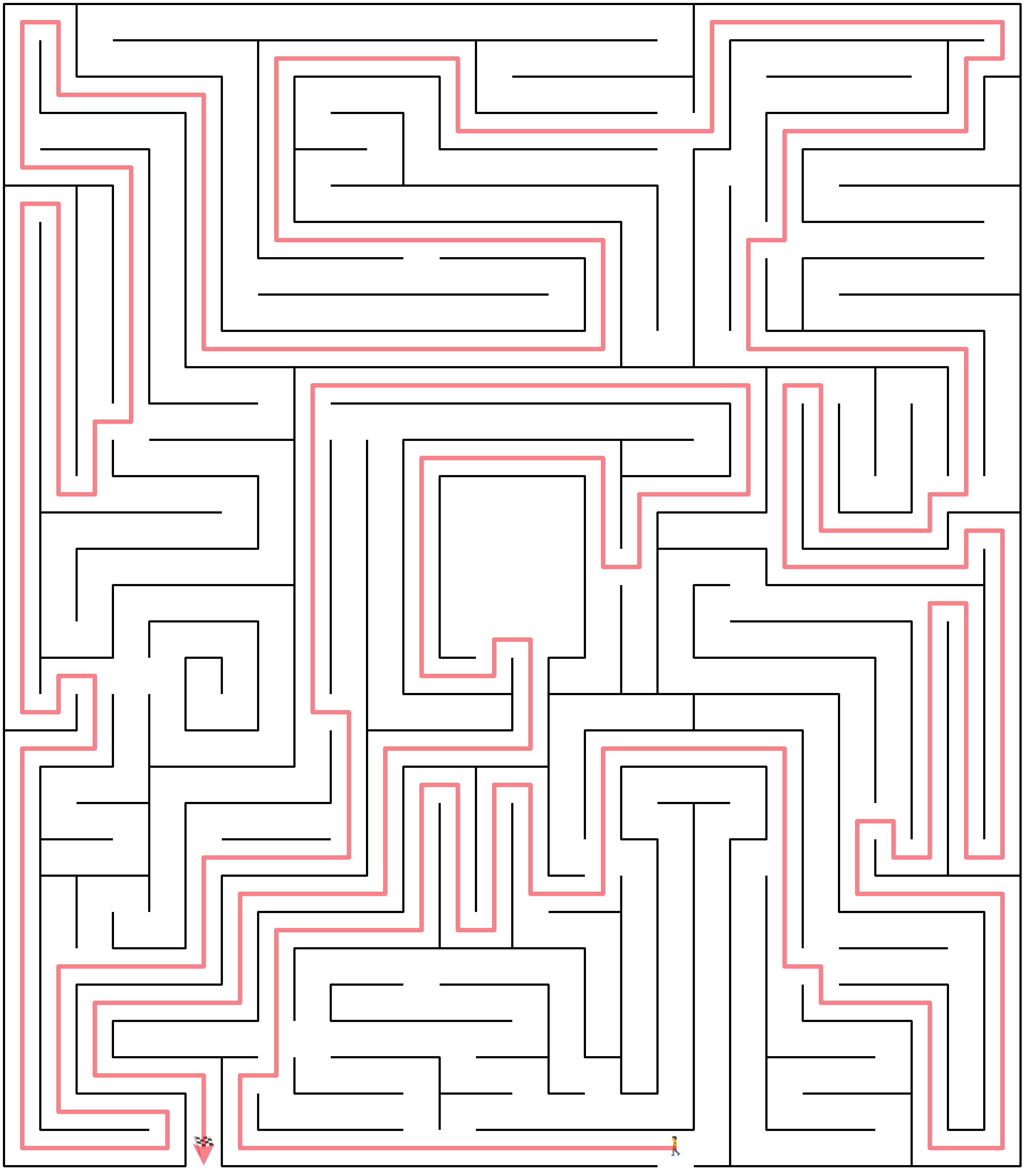
Its solution has 121 nodes, which looks impressive! However, there’s a flaw in how you currently compute the shortest path, whose length depends on the number of nodes in the graph instead of the number of squares in each path segment. This results in a solution that isn’t the shortest path in terms of actual distance. You’ll address this problem by adding edge weights shortly.
But there’s another problem. You’re currently unable to distinguish between multiple equivalent solutions. What if the maze had several paths with equal lengths? In such a case, you can call nx.all_shortest_paths(), which will return an iterator of the shortest paths in the graph:
# graphs/solver.py

import networkx as nx

from maze_solver.graphs.converter import make_graph
from maze_solver.models.maze import Maze
from maze_solver.models.solution import Solution

def solve(maze: Maze) -> Solution | None:
    try:
        return Solution(
            squares=tuple(
                nx.shortest_path(
                    make_graph(maze),
                    source=maze.entrance,
                    target=maze.exit,
                )
            )
        )
    except nx.NetworkXException:
        return None

def solve_all(maze: Maze) -> list[Solution]:
    try:
        return [
            Solution(squares=tuple(path))
            for path in nx.all_shortest_paths(
                make_graph(maze),
                source=maze.entrance,
                target=maze.exit,
            )
        ]
    except nx.NetworkXException:
        return []
Your solve_all() function wraps each yielded path in a Solution instance using a list comprehension or returns an empty list if no solution exists.
If you forget about the enemies and rewards for a moment, then the Pac-Man maze that you saw in the beginning of the tutorial has two alternative solutions. One goes through the top of the maze, and the other goes through the bottom. However, if you were to run solve_all() on such a maze, then you’d still only get one solution. Why?
The problem is that NetworkX calculates the cost of a solution based on the total number of nodes on its path, which may include intersections, corners, and other nodes that don’t actually increase the distance in any way. This may sometimes trick the shortest path algorithm into favoring alternative paths with equal distances but fewer nodes.
To fix that, you’re going to calculate the distance based on the actual number of squares in the maze along the path instead of the number of nodes in the graph. To convey the computed distance to NetworkX, you’ll add numeric weights to your graph edges.
Add Weights to Graph Edges
Go back to your converter module and update the Edge class by adding a property that’ll calculate the actual distance between its two nodes:
# graphs/converter.py

import math
from typing import NamedTuple, TypeAlias

import networkx as nx

from maze_solver.models.border import Border
from maze_solver.models.maze import Maze
from maze_solver.models.role import Role
from maze_solver.models.square import Square

Node: TypeAlias = Square

class Edge(NamedTuple):
    node1: Node
    node2: Node

    @property
    def distance(self) -> float:
        return math.dist(
            (self.node1.row, self.node1.column),
            (self.node2.row, self.node2.column)
        )

# ...
You calculate the Euclidean distance between the nodes using Python’s math module, whose dist() function takes two points specified as sequences of coordinates. In this case, you provide tuples of the row and column indices of squares corresponding to the nodes. Note that you could define distance differently—for example, as the sum of absolute values of differences in the horizontal and vertical directions.
You can update the function make_graph() below to use your new property:
# graphs/converter.py

# ...

def make_graph(maze: Maze) -> nx.Graph:
    return nx.Graph(
        (edge.node1, edge.node2, {"weight": edge.distance})
        for edge in get_edges(maze, get_nodes(maze))
    )

# ...
Notice how you changed the graph data passed to nx.Graph, which is now a sequence of tuples consisting of the two nodes and a dictionary with extra attributes. You specify only one attribute named weight, whose value is equal to the edge’s distance.
Next, you should update the functions in the solver module to tell NetworkX which attribute to use as the weight:
# graphs/solver.py

import networkx as nx

from maze_solver.graphs.converter import make_graph
from maze_solver.models.maze import Maze
from maze_solver.models.solution import Solution

def solve(maze: Maze) -> Solution | None:
    try:
        return Solution(
            squares=tuple(
                nx.shortest_path(
                    make_graph(maze),
                    source=maze.entrance,
                    target=maze.exit,
                    weight="weight",
                )
            )
        )
    except nx.NetworkXException:
        return None

def solve_all(maze: Maze) -> list[Solution]:
    try:
        return [
            Solution(squares=tuple(path))
            for path in nx.all_shortest_paths(
                make_graph(maze),
                source=maze.entrance,
                target=maze.exit,
                weight="weight",
            )
        ]
    except nx.NetworkXException:
        return []
The weight parameter lets you specify the name of an attribute in the dictionary associated with each graph edge.
Now, when you call solve_all() on the Pac-Man maze, you’ll get two equivalent solutions, which lead you to the exit on the left:
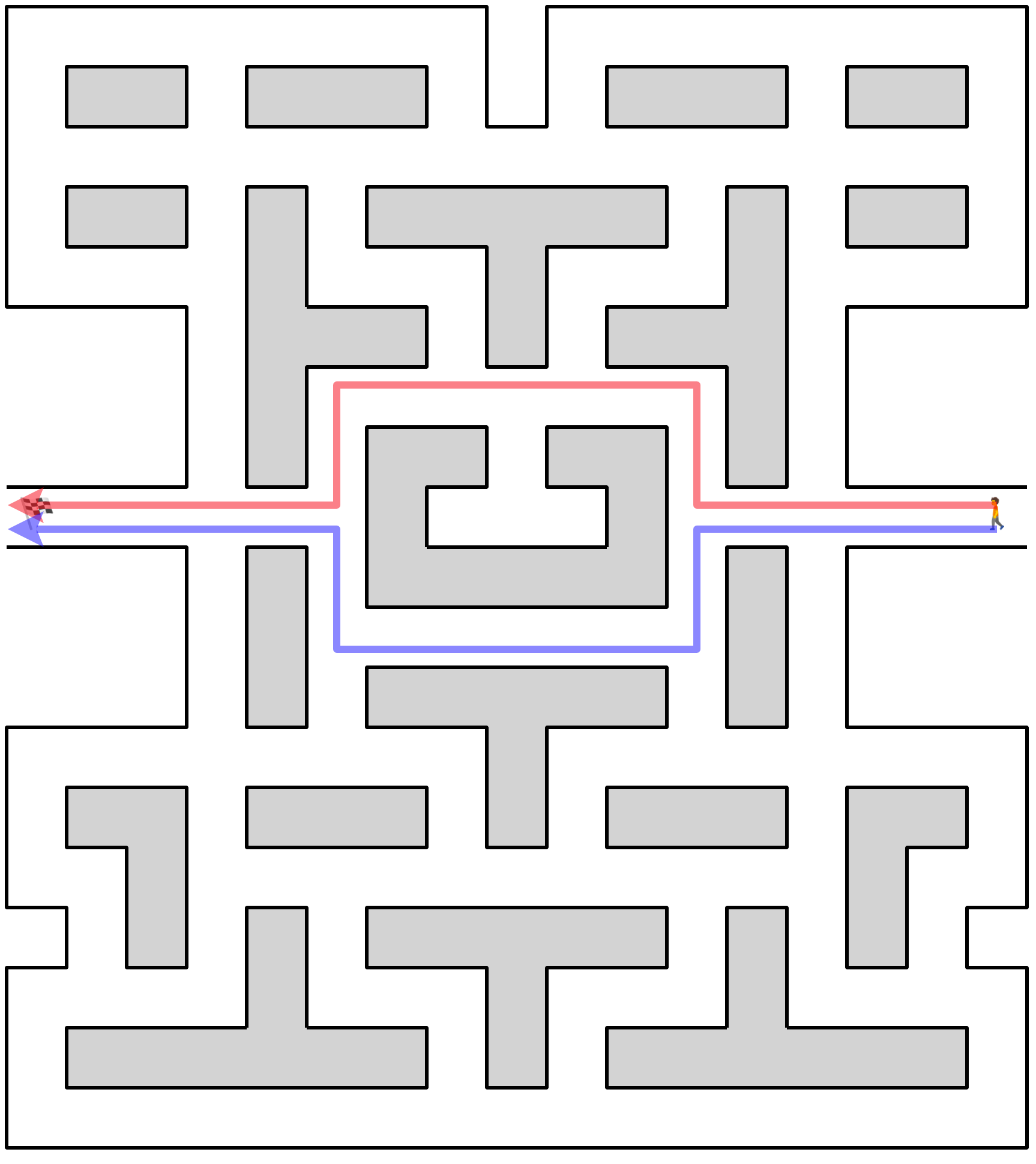
Clearly, both paths have the same length, so it shouldn’t matter which one you choose. However, notice that the upper path contains three extra nodes representing the intersections, including one with a chamber opening in the middle of the maze, while the lower path doesn’t.
Fantastic! Now that you have weights in your graph, you can use other factors besides the distance to influence the algorithm’s decision. For example, you may want to favor paths with fewer enemies or more rewards. You’ll find out how in the next section.
Introduce Enemies and Rewards to the Maze
Instead of using pure distance as an edge weight to assess how good a path is, you can take enemies and rewards into account to encourage or discourage certain paths in your maze.
Because you already recorded squares with special roles, including rewards and enemies, as nodes in your graph, you can assume they’ll be present at either end of an edge. This means that you don’t have to consider the squares that possibly exist between a pair of nodes connected by an edge.
The smaller the weight, the lower the cost of the edge connecting two nodes. Therefore, you can assign a lower weight to edges that pass through a reward. This will cause the algorithm to prioritize such paths over others. Conversely, you can set a higher weight to edges leading to undesirable destinations. Giving a penalty for enemies will make the algorithm avoid these paths.
You must carefully consider the scale and distribution of your edge weights. In particular, you shouldn’t have any negative weights in the graph because Dijkstra’s algorithm, which NetworkX uses by default, can’t cope with them. While you could try using the Bellman-Ford algorithm instead, it’ll fail as soon as it finds a negative cycle in your graph, whose edges add up to a negative value. So, it’s best to avoid negative weights altogether.
Note: To check if your graph contains negative weights, you can call nx.is_negatively_weighted() on the NetworkX graph object.
How you assign the weights depends on the specific problem. You may need to experiment a little, but in this tutorial, you’re going to follow a few rules, illustrated below:
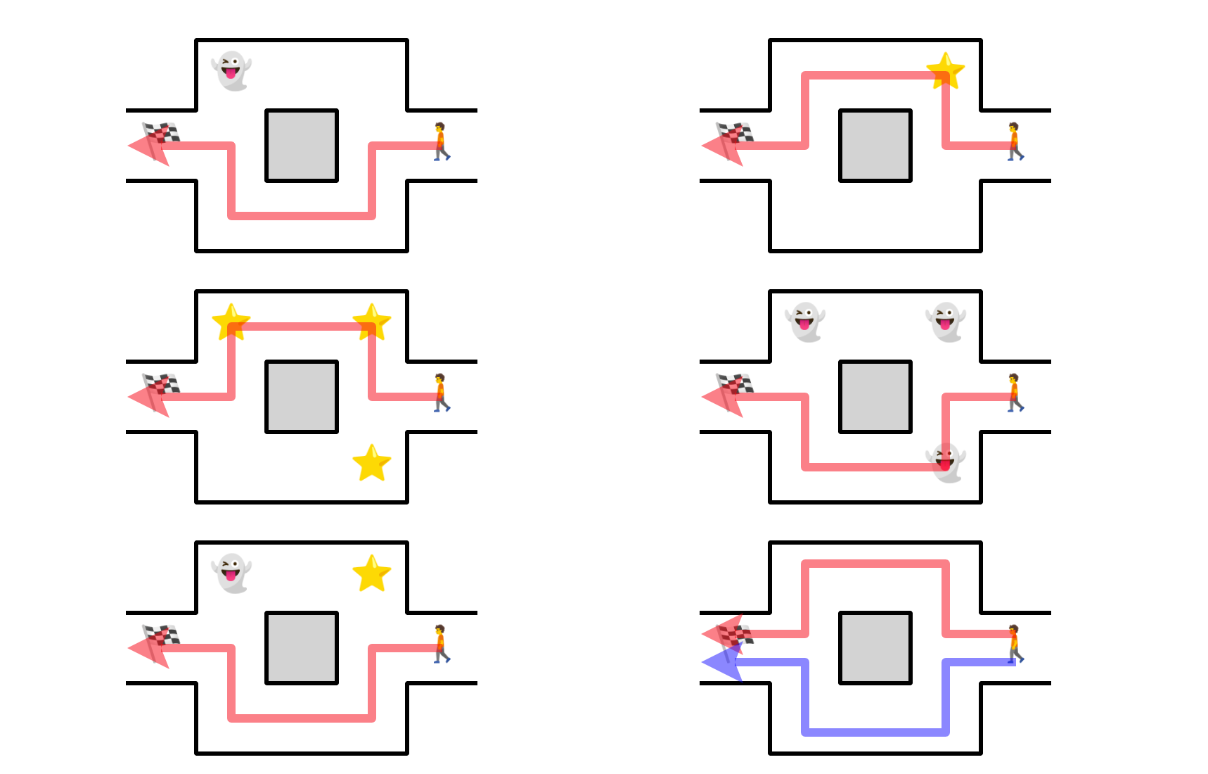
In plain English, you want to:
- Avoid enemies and seek rewards
- Given two paths with equal lengths, prefer one with more rewards
- Unless there’s no other choice, follow a path with fewer enemies
- If a path contains both a reward and an enemy, then give it a lower priority compared to an equivalent path without any rewards or enemies
- Use the distance between an edge’s nodes as the baseline weight, measured in squares in the maze
One way to achieve such an effect is to turn your maze into a directed graph and tie the edge weights to their target nodes, scaled by some arbitrary bonus and penalty points.
For example, you can subtract one bonus point from an edge’s weight for each reward while adding two penalty points for each enemy. This will always penalize enemies more than reward bonuses, giving the algorithm a preference for safer paths at the cost of potentially missing out on rewards.
To ensure that all edge weights are greater than zero, you could offset them so that the lowest weight is always positive. Unfortunately, adding a fixed offset to the weights would again make them depend on the number of superfluous nodes in the graph rather than the actual distance in the maze. Therefore, you won’t go down that rabbit hole.
Instead, you’ll implement the following method in your Edge class to calculate the weight of a directed edge:
# graphs/converter.py

import math
from typing import NamedTuple, TypeAlias

import networkx as nx

from maze_solver.models.border import Border
from maze_solver.models.maze import Maze
from maze_solver.models.role import Role
from maze_solver.models.square import Square

Node: TypeAlias = Square

class Edge(NamedTuple):
    node1: Node
    node2: Node

    @property
    def distance(self) -> int:
        return math.dist(
            (self.node1.row, self.node1.column),
            (self.node2.row, self.node2.column)
        )

    def weight(self, bonus=1, penalty=2) -> float:
        match self.node2.role:
            case Role.REWARD:
                return self.distance - bonus
            case Role.ENEMY:
                return self.distance + penalty
            case _:
                return self.distance

# ...
By default, this method subtracts one point from the baseline distance if the current edge leads to a reward. On the other hand, if there’s an enemy at the end of this edge, then the method adds two penalty points to increase the cost of that connection. Otherwise, the weight of an edge is equal to its distance.
Note: When both nodes connected by an edge are located on adjacent squares in the maze, the minimum distance is equal to one unit.
Feel free to tweak the bonus and penalty points to your liking—for example, to favor even more distant rewards, making bigger detours from the shortest path worthwhile. However, note that while you can safely bump up penalty points, using more bonus points will increase the risk of ending up with a negative weight, which would lead to an error.
At the moment, the graph you made is undirected, meaning you can’t know whether the search algorithm is moving towards the first or the second node in the edge. Go ahead and replace it with a directed graph, using your new method as the weight:
# graphs/converter.py

# ...

class Edge(NamedTuple):
    node1: Node
    node2: Node

    @property
    def flip(self) -> "Edge":
        return Edge(self.node2, self.node1)

    # ...

def make_graph(maze: Maze) -> nx.DiGraph:
    return nx.DiGraph(
        (edge.node1, edge.node2, {"weight": edge.weight()})
        for edge in get_directed_edges(maze, get_nodes(maze))
    )

def get_directed_edges(maze: Maze, nodes: set[Node]) -> set[Edge]:
    return (edges := get_edges(maze, nodes)) | {edge.flip for edge in edges}

# ...
The .flip property of an edge returns a new Edge instance with its two nodes reversed. You use it in get_directed_edges() below to return a set of edges in both directions based on the undirected edges. Depending on the direction, the same edge may have different weights. Finally, you create an nx.DiGraph object instead of nx.Graph to represent the graph as directed.
To put your new weights to the test, try solving the sample mazes, but this time, add enemies and rewards into them. You can streamline this process by first making your maze_solver package runnable.
Make a Runnable Script
In this section, you’ll provide a command-line interface with argparse to your Python package. It’ll take a path to a binary file with your maze as input. Then, it’ll try to find the maze’s solutions and render them in separate tabs in your web browser as scalable vector graphics. On the other hand, if it can’t find any solutions, then you’ll see an appropriate message in your console.
Add the special __main__.py file in your project to turn it into a runnable Python package:
maze-solver/
│
├── src/
│   │
│   └── maze_solver/
│       │
│       ├── graphs/
│       │   ├── __init__.py
│       │   ├── converter.py
│       │   └── solver.py
│       │
│       ├── models/
│       │   ├── __init__.py
│       │   ├── border.py
│       │   ├── maze.py
│       │   ├── role.py
│       │   ├── solution.py
│       │   └── square.py
│       │
│       ├── persistence/
│       │   ├── __init__.py
│       │   ├── file_format.py
│       │   └── serializer.py
│       │
│       ├── view/
│       │   ├── __init__.py
│       │   ├── decomposer.py
│       │   ├── primitives.py
│       │   └── renderer.py
│       │
│       ├── __init__.py
│       └── __main__.py
│
├── pyproject.toml
└── requirements.txt
The file should live inside your maze_solver package, next to the empty __init__.py file. Its contents should look as follows:
# __main__.py

import argparse
import pathlib

from maze_solver.graphs.solver import solve_all
from maze_solver.models.maze import Maze
from maze_solver.view.renderer import SVGRenderer

def main() -> None:
    maze = Maze.load(parse_path())
    solutions = solve_all(maze)
    if solutions:
        renderer = SVGRenderer()
        for solution in solutions:
            renderer.render(maze, solution).preview()
    else:
        print("No solution found")

def parse_path() -> pathlib.Path:
    parser = argparse.ArgumentParser()
    parser.add_argument("path", type=pathlib.Path)
    return parser.parse_args().path

if __name__ == "__main__":
    main()
The file uses the name-main idiom to protect the main() function from running if other modules import the package. It uses the argparse module to parse the file path, which is currently the only expected command-line argument. Later, you can add more if you want to, for example, allow for previewing mazes without a solution. Finally, the code finds, renders, and previews all the solutions of the loaded maze or prints an error message.
To run this package, you can issue the following command in your terminal:
(venv) $ python -m maze_solver /path/to/file.maze
However, you can optionally specify a handy shortcut in your pyproject.toml file:
# pyproject.toml

[build-system]
requires = ["setuptools>=64.0.0", "wheel"]
build-backend = "setuptools.build_meta"

[project]
name = "maze-solver"
version = "1.0.0"

dependencies = [
    "networkx == 3.0",
]

[project.scripts]
solve = "maze_solver.__main__:main"
You may have as many custom commands like this as you like, which should map to specific functions in the given module within your project. To register the new command in your virtual environment, you must install the package using pip again:
(venv) $ python -m pip install -e .
When you reinstall the package, you’ll be able to solve mazes using the solve command without explicitly calling out Python:
(venv) $ solve /path/to/file.maze
Note that you need to run it from your virtual environment. The solve command, which you just created, isn’t available outside of it!
Great, now you have a working command-line interface to your Python package. While there are no further steps in this tutorial, you can always keep improving the project. For example, you may add more command-line arguments to control the rendering process or provide an option to save the results as an image instead of previewing them in the browser. The possibilities are endless!
Conclusion
Congratulations on completing this in-depth tutorial!
You’ve successfully built a maze solver in Python, which you can use to find one or more solutions to mazes stored in your custom binary file format. You know how to represent the maze both in object-oriented and graph form suitable for the NetworkX library and how to visualize it using scalable vector graphics. Finally, you made a self-contained, runnable Python package with a command-line interface.
In this tutorial, you’ve learned how to:
- Use an object-oriented approach to represent the maze in memory
- Define a specialized binary file format to store the maze on disk
- Transform the maze into a traversable weighted graph
- Use graph search algorithms in the NetworkX library to find the solution
- Visualize the maze and its solution using scalable vector graphics (SVG)
You can find the complete source code for this project, as well as snapshots of the individual steps, in the supporting materials, which you can download using the link below:
Free Download: Click here to download the source code and supporting materials that you’ll use to build a maze solver in Python.
Watch Now This tutorial has a related video course created by the Real Python team. Watch it together with the written tutorial to deepen your understanding: Mazes in Python: Build, Visualize, Store, and Solve