Are you a Python developer brushing up on your skills before an interview? If so, then this tutorial will usher you through a series of Python practice problems meant to simulate common coding test scenarios. After you develop your own solutions, you’ll walk through the Real Python team’s answers so you can optimize your code, impress your interviewer, and land your dream job!
In this tutorial, you’ll learn how to:
- Write code for interview-style problems
- Discuss your solutions during the interview
- Work through frequently overlooked details
- Talk about design decisions and trade-offs
This tutorial is aimed at intermediate Python developers. It assumes a basic knowledge of Python and an ability to solve problems in Python. You can get skeleton code with failing unit tests for each of the problems you’ll see in this tutorial by clicking on the link below:
Download the sample code: Click here to get the code you’ll use to work through the Python practice problems in this tutorial.
Each of the problems below shows the file header from this skeleton code describing the problem requirements. So download the code, fire up your favorite editor, and let’s dive into some Python practice problems!
Python Practice Problem 1: Sum of a Range of Integers
Let’s start with a warm-up question. In the first practice problem, you’ll write code to sum a list of integers. Each practice problem includes a problem description. This description is pulled directly from the skeleton files in the repo to make it easier to remember while you’re working on your solution.
You’ll see a solution section for each problem as well. Most of the discussion will be in a collapsed section below that. Clone that repo if you haven’t already, work out a solution to the following problem, then expand the solution box to review your work.
Problem Description
Here’s your first problem:
Sum of Integers Up To n (
integersums.py)Write a function,
add_it_up(), that takes a single integer as input and returns the sum of the integers from zero to the input parameter.The function should return 0 if a non-integer is passed in.
Remember to run the unit tests until you get them passing!
Problem Solution
Here’s some discussion of a couple of possible solutions.
Note: Remember, don’t open the collapsed section below until you’re ready to look at the answer for this Python practice problem!
How did writing the solution go? Ready to look at the answer?
For this problem, you’ll look at a few different solutions. The first of these is not so good:
# integersums.py
def first(n):
    num = 1
    sum = 0
    while num < n + 1:
        sum = sum + num
        num = num + 1
    return sum
In this solution, you manually build a while loop to run through the numbers 1 through n. You keep a running sum and then return it when you’ve finished the loop.
This solution works, but it has two problems:
-
It doesn’t display your knowledge of Python and how the language simplifies tasks like this.
-
It doesn’t meet the error conditions in the problem description. Passing in a string will result in the function throwing an exception when it should just return
0.
You’ll deal with the error conditions in the final answer below, but first let’s refine the core solution to be a bit more Pythonic.
The first thing to think about is that while loop. Python has powerful mechanisms for iterating over lists and ranges. Creating your own is usually unnecessary, and that’s certainly the case here. You can replace the while loop with a loop that iterates over a range():
# integersums.py
def better(n):
    sum = 0
    for num in range(n + 1):
        sum += num
    return sum
You can see that the for...range() construct has replaced your while loop and shortened the code. One thing to note is that range() goes up to but does not include the number given, so you need to use n + 1 here.
This was a nice step! It removes some of the boilerplate code of looping over a range and makes your intention clearer. But there’s still more you can do here.
Summing a list of integers is another thing Python is good at:
# integersums.py
def even_better(n):
    return sum(range(n + 1))
Wow! By using the built-in sum(), you got this down to one line of code! While code golf generally doesn’t produce the most readable code, in this case you have a win-win: shorter and more readable code.
There’s one problem remaining, however. This code still doesn’t handle the error conditions correctly. To fix that, you can wrap your previous code in a try...except block:
# integersums.py
def add_it_up(n):
    try:
        result = sum(range(n + 1))
    except TypeError:
        result = 0
    return result
This solves the problem and handles the error conditions correctly. Way to go!
Occasionally, interviewers will ask this question with a fixed limit, something like “Print the sum of the first nine integers.” When the problem is phrased that way, one correct solution would be print(45).
If you give this answer, however, then you should follow up with code that solves the problem step by step. The trick answer is a good place to start your answer, but it’s not a great place to end.
If you’d like to extend this problem, try adding an optional lower limit to add_it_up() to give it more flexibility!
Python Practice Problem 2: Caesar Cipher
The next question is a two-parter. You’ll code up a function to compute a Caesar cipher on text input. For this problem, you’re free to use any part of the Python standard library to do the transform.
Hint: There’s a function in the str class that will make this task much easier!
Problem Description
The problem statement is at the top of the skeleton source file:
Caesar Cipher (
caesar.py)A Caesar cipher is a simple substitution cipher in which each letter of the plain text is substituted with a letter found by moving
nplaces down the alphabet. For example, assume the input plain text is the following:abcd xyzIf the shift value,
n, is 4, then the encrypted text would be the following:efgh bcdYou are to write a function that accepts two arguments, a plain-text message and a number of letters to shift in the cipher. The function will return an encrypted string with all letters transformed and all punctuation and whitespace remaining unchanged.
Note: You can assume the plain text is all lowercase ASCII except for whitespace and punctuation.
Remember, this part of the question is really about how well you can get around in the standard library. If you find yourself figuring out how to do the transform without the library, then save that thought! You’ll need it later!
Problem Solution
Here’s a solution to the Caesar cipher problem described above.
Note: Remember, don’t open the collapsed section below until you’re ready to look at the answers for this Python practice problem!
This solution makes use of .translate() from the str class in the standard library. If you struggled with this problem, then you might want to pause a moment and consider how you could use .translate() in your solution.
Okay, now that you’re ready, let’s look at this solution:
 1# caesar.py
 2import string
 3
 4def caesar(plain_text, shift_num=1):
 5    letters = string.ascii_lowercase
 6    mask = letters[shift_num:] + letters[:shift_num]
 7    trantab = str.maketrans(letters, mask)
 8    return plain_text.translate(trantab)
You can see that the function makes use of three things from the string module:
.ascii_lowercase.maketrans().translate()
In the first two lines, you create a variable with all the lowercase letters of the alphabet (ASCII only for this program) and then create a mask, which is the same set of letters, only shifted. The slicing syntax is not always obvious, so let’s walk through it with a real-world example:
>>> import string
>>> x = string.ascii_lowercase
>>> x
'abcdefghijklmnopqrstuvwxyz'
>>> x[3:]
'defghijklmnopqrstuvwxyz'
>>> x[:3]
'abc'
You can see that x[3:] is all the letters after the third letter, 'c', while x[:3] is just the first three letters.
Line 6 in the solution, letters[shift_num:] + letters[:shift_num], creates a list of letters shifted by shift_num letters, with the letters at the end wrapped around to the front. Once you have the list of letters and the mask of letters you want to map to, you call .maketrans() to create a translation table.
Next, you pass the translation table to the string method .translate(). It maps all characters in letters to the corresponding letters in mask and leaves all other characters alone.
This question is an exercise in knowing and using the standard library. You may be asked a question like this at some point during an interview. If that happens to you, it’s good to spend some time thinking about possible answers. If you can remember the method—.translate() in this case—then you’re all set.
But there are a couple of other scenarios to consider:
-
You may completely draw a blank. In this case, you’ll probably solve this problem the way you solve the next one, and that’s an acceptable answer.
-
You may remember that the standard library has a function to do what you want but not remember the details.
If you were doing normal work and hit either of these situations, then you’d just do some searching and be on your way. But in an interview situation, it will help your cause to talk through the problem out loud.
Asking the interviewer for specific help is far better than just ignoring it. Try something like “I think there’s a function that maps one set of characters to another. Can you help me remember what it’s called?”
In an interview situation, it’s often better to admit that you don’t know something than to try to bluff your way through.
Now that you’ve seen a solution using the Python standard library, let’s try the same problem again, but without that help!
Python Practice Problem 3: Caesar Cipher Redux
For the third practice problem, you’ll solve the Caesar cipher again, but this time you’ll do it without using .translate().
Problem Description
The description of this problem is the same as the previous problem. Before you dive into the solution, you might be wondering why you’re repeating the same exercise, just without the help of .translate().
That’s a great question. In normal life, when your goal is to get a working, maintainable program, rewriting parts of the standard library is a poor choice. The Python standard library is packed with working, well-tested, and fast solutions for problems large and small. Taking full advantage of it is a mark of a good programmer.
That said, this is not a work project or a program you’re building to satisfy a need. This is a learning exercise, and it’s the type of question that might be asked during an interview. The goal for both is to see how you can solve the problem and what interesting design trade-offs you make while doing it.
So, in the spirit of learning, let’s try to resolve the Caesar cipher without .translate().
Problem Solution
For this problem, you’ll have two different solutions to look at when you’re ready to expand the section below.
Note: Remember, don’t open the collapsed section below until you’re ready to look at the answers for this Python practice problem!
For this problem, two different solutions are provided. Check out both and see which one you prefer!
Solution 1
For the first solution, you follow the problem description closely, adding an amount to each character and flipping it back to the beginning of the alphabet when it goes on beyond z:
 1# caesar.py
 2import string
 3
 4def shift_n(letter, amount):
 5    if letter not in string.ascii_lowercase:
 6        return letter
 7    new_letter = ord(letter) + amount
 8    while new_letter > ord("z"):
 9        new_letter -= 26
10    while new_letter < ord("a"):
11        new_letter += 26
12    return chr(new_letter)
13
14def caesar(message, amount):
15    enc_list = [shift_n(letter, amount) for letter in message]
16    return "".join(enc_list)
Starting on line 14, you can see that caesar() does a list comprehension, calling a helper function for each letter in message. It then does a .join() to create the new encoded string. This is short and sweet, and you’ll see a similar structure in the second solution. The interesting part happens in shift_n().
Here you can see another use for string.ascii_lowercase, this time filtering out any letter that isn’t in that group. Once you’re certain you’ve filtered out any non-letters, you can proceed to encoding. In this version of encoding, you use two functions from the Python standard library:
Again, you’re encouraged not only to learn these functions but also to consider how you might respond in an interview situation if you couldn’t remember their names.
ord() does the work of converting a letter to a number, and chr() converts it back to a letter. This is handy as it allows you to do arithmetic on letters, which is what you want for this problem.
The first step of your encoding on line 7 gets the numeric value of the encoded letter by using ord() to get the numeric value of the original letter. ord() returns the Unicode code point of the character, which turns out to be the ASCII value.
For many letters with small shift values, you can convert the letter back to a character and you’ll be done. But consider the starting letter, z.
A shift of one character should result in the letter a. To achieve this wraparound, you find the difference from the encoded letter to the letter z. If that difference is positive, then you need to wrap back to the beginning.
You do this in lines 8 to 11 by repeatedly adding 26 to or subtracting it from the character until it’s in the range of ASCII characters. Note that this is a fairly inefficient method for fixing this issue. You’ll see a better solution in the next answer.
Finally, on line 12, your conversion shift function takes the numeric value of the new letter and converts it back to a letter to return it.
While this solution takes a literal approach to solving the Caesar cipher problem, you could also use a different approach modeled after the .translate() solution in practice problem 2.
Solution 2
The second solution to this problem mimics the behavior of Python’s built-in method .translate(). Instead of shifting each letter by a given amount, it creates a translation map and uses it to encode each letter:
 1# caesar.py
 2import string
 3
 4def shift_n(letter, table):
 5    try:
 6        index = string.ascii_lowercase.index(letter)
 7        return table[index]
 8    except ValueError:
 9        return letter
10
11def caesar(message, amount):
12    amount = amount % 26
13    table = string.ascii_lowercase[amount:] + string.ascii_lowercase[:amount]
14    enc_list = [shift_n(letter, table) for letter in message]
15    return "".join(enc_list)
Starting with caesar() on line 11, you start by fixing the problem of amount being greater than 26. In the previous solution, you looped repeatedly until the result was in the proper range. Here, you take a more direct and more efficient approach using the mod operator (%).
The mod operator produces the remainder from an integer division. In this case, you divide by 26, which means the results are guaranteed to be between 0 and 25, inclusive.
Next, you create the translation table. This is a change from the previous solutions and is worth some attention. You’ll see more about this toward the end of this section.
Once you create the table, the rest of caesar() is identical to the previous solution: a list comprehension to encrypt each letter and a .join() to create a string.
shift_n() finds the index of the given letter in the alphabet and then uses this to pull a letter from the table. The try...except block catches those cases that aren’t found in the list of lowercase letters.
Now let’s discuss the table creation issue. For this toy example, it probably doesn’t matter too much, but it illustrates a situation that occurs frequently in everyday development: balancing clarity of code against known performance bottlenecks.
If you examine the code again, you’ll see that table is used only inside shift_n(). This indicates that, in normal circumstances, it should have been created in, and thus have its scope limited to, shift_n():
# caesar.py
import string

def slow_shift_n(letter, amount):
    table = string.ascii_lowercase[amount:] + string.ascii_lowercase[:amount]
    try:
        index = string.ascii_lowercase.index(letter)
        return table[index]
    except ValueError:
        return letter

def slow_caesar(message, amount):
    amount = amount % 26
    enc_list = [shift_n(letter, amount) for letter in message]
    return "".join(enc_list)
The issue with that approach is that it spends time calculating the same table for every letter of the message. For small messages, this time will be negligible, but it might add up for larger messages.
Another possible way that you could avoid this performance penalty would be to make table a global variable. While this also cuts down on the construction penalty, it makes the scope of table even larger. This doesn’t seem better than the approach shown above.
At the end of the day, the choice between creating table once up front and giving it a larger scope or just creating it for every letter is what’s called a design decision. You need to choose the design based on what you know about the actual problem you’re trying to solve.
If this is a small project and you know it will be used to encode large messages, then creating the table only once could be the right decision. If this is only a portion of a larger project, meaning maintainability is key, then perhaps creating the table each time is the better option.
Since you’ve looked at two solutions, it’s worth taking a moment to discuss their similarities and differences.
Solution Comparison
You’ve seen two solutions in this part of the Caesar cipher, and they’re fairly similar in many ways. They’re about the same number of lines. The two main routines are identical except for limiting amount and creating table. It’s only when you look at the two versions of the helper function, shift_n(), that the differences appear.
The first shift_n() is an almost literal translation of what the problem is asking for: “Shift the letter down the alphabet and wrap it around at z.” This clearly maps back to the problem statement, but it has a few drawbacks.
Although it’s about the same length as the second version, the first version of shift_n() is more complex. This complexity comes from the letter conversion and math needed to do the translation. The details involved—converting to numbers, subtracting, and wrapping—mask the operation you’re performing. The second shift_n() is far less involved in its details.
The first version of the function is also specific to solving this particular problem. The second version of shift_n(), like the standard library’s .translate() that it’s modeled after, is more general-purpose and can be used to solve a larger set of problems. Note that this is not necessarily a good design goal.
One of the mantras that came out of the Extreme Programming movement is “You aren’t gonna need it” (YAGNI). Frequently, software developers will look at a function like shift_n() and decide that it would be better and more general-purpose if they made it even more flexible, perhaps by passing in a parameter instead of using string.ascii_lowercase.
While that would indeed make the function more general-purpose, it would also make it more complex. The YAGNI mantra is there to remind you not to add complexity before you have a specific use case for it.
To wrap up your Caesar cipher section, there are clear trade-offs between the two solutions, but the second shift_n() seems like a slightly better and more Pythonic function.
Now that you’ve written the Caesar cipher three different ways, let’s move on to a new problem.
Python Practice Problem 4: Log Parser
The log parser problem is one that occurs frequently in software development. Many systems produce log files during normal operation, and sometimes you’ll need to parse these files to find anomalies or general information about the running system.
Problem Description
For this problem, you’ll need to parse a log file with a specified format and generate a report:
Log Parser (
logparse.py)Accepts a filename on the command line. The file is a Linux-like log file from a system you are debugging. Mixed in among the various statements are messages indicating the state of the device. They look like this:
Jul 11 16:11:51:490 [139681125603136] dut: Device State: ONThe device state message has many possible values, but this program cares about only three:
ON,OFF, andERR.Your program will parse the given log file and print out a report giving how long the device was
ONand the timestamp of anyERRconditions.
Note that the provided skeleton code doesn’t include unit tests. This was omitted since the exact format of the report is up to you. Think about and write your own during the process.
A test.log file is included, which provides you with an example. The solution you’ll examine produces the following output:
$ ./logparse.py test.log
Device was on for 7 seconds
Timestamps of error events:
   Jul 11 16:11:54:661
   Jul 11 16:11:56:067
While that format is generated by the Real Python solution, you’re free to design your own format for the output. The sample input file should generate equivalent information.
Problem Solution
In the collapsed section below, you’ll find a possible solution to the log parser problem. When you’re ready, expand the box and compare it with what you came up with!
Note: Remember, don’t open the collapsed section below until you’re ready to look at the answers for this Python practice problem!
Full Solution
Since this solution is longer than what you saw for the integer sums or the Caesar cipher problems, let’s start with the full program:
# logparse.py
import datetime
import sys

def get_next_event(filename):
    with open(filename, "r") as datafile:
        for line in datafile:
            if "dut: Device State: " in line:
                line = line.strip()
                # Parse out the action and timestamp
                action = line.split()[-1]
                timestamp = line[:19]
                yield (action, timestamp)

def compute_time_diff_seconds(start, end):
    format = "%b %d %H:%M:%S:%f"
    start_time = datetime.datetime.strptime(start, format)
    end_time = datetime.datetime.strptime(end, format)
    return (end_time - start_time).total_seconds()

def extract_data(filename):
    time_on_started = None
    errs = []
    total_time_on = 0

    for action, timestamp in get_next_event(filename):
        # First test for errs
        if "ERR" == action:
            errs.append(timestamp)
        elif ("ON" == action) and (not time_on_started):
            time_on_started = timestamp
        elif ("OFF" == action) and time_on_started:
            time_on = compute_time_diff_seconds(time_on_started, timestamp)
            total_time_on += time_on
            time_on_started = None
    return total_time_on, errs

if __name__ == "__main__":
    total_time_on, errs = extract_data(sys.argv[1])
    print(f"Device was on for {total_time_on} seconds")
    if errs:
        print("Timestamps of error events:")
        for err in errs:
            print(f"\t{err}")
    else:
        print("No error events found.")
That’s your full solution. You can see that the program consists of three functions and the main section. You’ll work through them from the top.
Helper Function: get_next_event()
First up is get_next_event():
# logparse.py
def get_next_event(filename):
    with open(filename, "r") as datafile:
        for line in datafile:
            if "dut: Device State: " in line:
                line = line.strip()
                # Parse out the action and timestamp
                action = line.split()[-1]
                timestamp = line[:19]
                yield (action, timestamp)
Because it contains a yield statement, this function is a generator. That means you can use it to generate one event from the log file at a time.
You could have just used for line in datafile, but instead you add a little bit of filtering. The calling routine will get only those events that have dut: Device State: in them. This keeps all the file-specific parsing contained in a single function.
This might make get_next_event() a bit more complicated, but it’s a relatively small function, so it remains short enough to read and comprehend. It also keeps that complicated code encapsulated in a single location.
You might be wondering when datafile gets closed. As long as you call the generator until all of the lines are read from datafile, the for loop will complete, allowing you to leave the with block and exit from the function.
Helper Function: compute_time_diff_seconds()
The second function is compute_time_diff_seconds(), which, as the name suggests, computes the number of seconds between two timestamps:
# logparse.py
def compute_time_diff_seconds(start, end):
    format = "%b %d %H:%M:%S:%f"
    start_time = datetime.datetime.strptime(start, format)
    end_time = datetime.datetime.strptime(end, format)
    return (end_time - start_time).total_seconds()
There are a few interesting points to this function. The first is that subtracting the two datetime objects results in a datetime.timedelta. For this problem, you will report total seconds, so returning .total_seconds() from the timedelta is appropriate.
The second item of note is that there are many, many packages in Python that simplify handling dates and times. In this case, your use model is simple enough that it doesn’t warrant the complexity of pulling in an external library when the standard library functions will suffice.
That said, datetime.datetime.strptime() is worthy of mention. When passed a string and a specific format,.strptime() parses that string with the given format and produces a datetime object.
This is another place where, in an interview situation, it’s important not to panic if you can’t remember the exact names of the Python standard library functions.
Helper Function: extract_data()
Next up is extract_data(), which does the bulk of the work in this program. Before you dive into the code, let’s step back and talk about state machines.
State machines are software (or hardware) devices that transition from one state to another depending on specific inputs. That’s a really broad definition that might be difficult to grasp, so let’s look at a diagram of the state machine you’ll be using below:
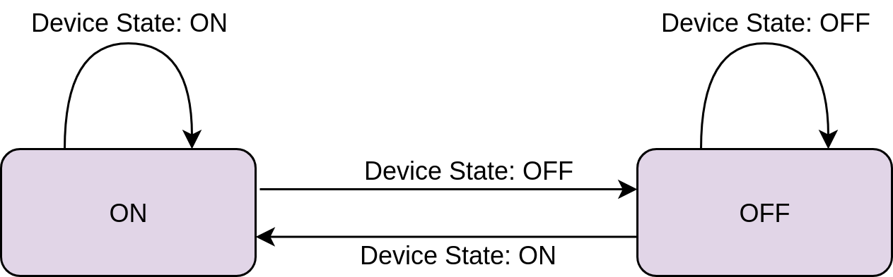
In this diagram, the states are represented by the labeled boxes. There are only two states here, ON and OFF, which correspond to the state of the device. There are also two input signals, Device State: ON and Device State: OFF. The diagram uses arrows to show what happens when an input occurs while the machine is in each state.
For example, if the machine is in the ON state and the Device State: ON input occurs, then the machine stays in the ON state. No change happens. Conversely, if the machine receives the Device State: OFF input when it’s in the ON state, then it will transition to the OFF state.
While the state machine here is only two states with two inputs, state machines are often much more complex. Creating a diagram of expected behavior can help you make the code that implements the state machine more concise.
Let’s move back to extract_data():
# logparse.py
def extract_data(filename):
    time_on_started = None
    errs = []
    total_time_on = 0

    for action, timestamp in get_next_event(filename):
        # First test for errs
        if "ERR" == action:
            errs.append(timestamp)
        elif ("ON" == action) and (not time_on_started):
            time_on_started = timestamp
        elif ("OFF" == action) and time_on_started:
            time_on = compute_time_diff_seconds(time_on_started, timestamp)
            total_time_on += time_on
            time_on_started = None
    return total_time_on, errs
It might be hard to see the state machine here. Usually, state machines require a variable to hold the state. In this case, you use time_on_started to serve two purposes:
- Indicate state:
time_on_startedholds the state of your state machine. If it’sNone, then the machine is in theOFFstate. If it’snot None, then the machine isON. - Store start time: If the state is
ON, thentime_on_startedalso holds the timestamp of when the device turned on. You use this timestamp to callcompute_time_diff_seconds().
The top of extract_data() sets up your state variable, time_on_started, and also the two outputs you want. errs is a list of timestamps at which the ERR message was found, and total_time_on is the sum of all periods when the device was on.
Once you’ve completed the initial setup, you call the get_next_event() generator to retrieve each event and timestamp. The action it receives is used to drive the state machine, but before it checks for state changes, it first uses an if block to filter out any ERR conditions and add those to errs.
After the error check, the first elif block handles transitions to the ON state. You can transition to ON only when you’re in the OFF state, which is signaled by time_on_started being False. If you’re not already in the ON state and the action is "ON", then you store the timestamp, putting the machine into the ON state.
The second elif handles the transition to the OFF state. On this transition, extract_data() needs to compute the number of seconds the device was on. It does this using the compute_time_diff_seconds() you saw above. It adds this time to the running total_time_on and sets time_on_started back to None, effectively putting the machine back into the OFF state.
Main Function
Finally, you can move on to the __main__ section. This final section passes sys.argv[1], which is the first command-line argument, to extract_data() and then presents a report of the results:
# logparse.py
if __name__ == "__main__":
    total_time_on, errs = extract_data(sys.argv[1])
    print(f"Device was on for {total_time_on} seconds")
    if errs:
        print("Timestamps of error events:")
        for err in errs:
            print(f"\t{err}")
    else:
        print("No error events found.")
To call this solution, you run the script and pass the name of the log file. Running your example code results in this output:
$ python3 logparse.py test.log
Device was on for 7 seconds
Timestamps of error events:
   Jul 11 16:11:54:661
   Jul 11 16:11:56:067
Your solution might have different formatting, but the information should be the same for the sample log file.
There are many ways to solve a problem like this. Remember that in an interview situation, talking through the problem and your thought process can be more important than which solution you choose to implement.
That’s it for the log-parsing solution. Let’s move on to the final challenge: sudoku!
Python Practice Problem 5: Sudoku Solver
Your final Python practice problem is to solve a sudoku puzzle!
Finding a fast and memory-efficient solution to this problem can be quite a challenge. The solution you’ll examine has been selected for readability rather than speed, but you’re free to optimize your solution as much as you want.
Problem Description
The description for the sudoku solver is a little more involved than the previous problems:
Sudoku Solver (
sudokusolve.py)Given a string in SDM format, described below, write a program to find and return the solution for the sudoku puzzle in the string. The solution should be returned in the same SDM format as the input.
Some puzzles will not be solvable. In that case, return the string “Unsolvable”.
The general SDM format is described here.
For our purposes, each SDM string will be a sequence of 81 digits, one for each position on the sudoku puzzle. Known numbers will be given, and unknown positions will have a zero value.
For example, assume you’re given this string of digits:
004006079000000602056092300078061030509000406020540890007410920105000000840600100The string represents this starting sudoku puzzle:
0 0 4   0 0 6   0 7 9
0 0 0   0 0 0   6 0 2
0 5 6   0 9 2   3 0 0

0 7 8   0 6 1   0 3 0
5 0 9   0 0 0   4 0 6
0 2 0   5 4 0   8 9 0

0 0 7   4 1 0   9 2 0
1 0 5   0 0 0   0 0 0
8 4 0   6 0 0   1 0 0
The provided unit tests may take a while to run, so be patient.
Note: A description of the sudoku puzzle can be found on Wikipedia.
You can see that you’ll need to deal with reading and writing to a particular format as well as generating a solution.
Problem Solution
When you’re ready, you can find a detailed explanation of a solution to the sudoku problem in the box below. A skeleton file with unit tests is provided in the repo.
Note: Remember, don’t open the collapsed section below until you’re ready to look at the answers for this Python practice problem!
This is a larger and more complex problem than you’ve looked at so far in this tutorial. You’ll walk through the problem step by step, ending with a recursive function that solves the puzzle. Here’s a rough outline of the steps you’ll take:
- Read the puzzle into a grid form.
- For each cell:
- For each possible number in that cell:
- Place the number in the cell.
- Remove that number from the row, column, and small square.
- Move to the next position.
- If no possible numbers remain, then declare the puzzle unsolvable.
- If all cells are filled, then return the solution.
- For each possible number in that cell:
The tricky part of this algorithm is keeping track of the grid at each step of the process. You’ll use recursion, making a new copy of the grid at each level of the recursion, to maintain this information.
With that outline in mind, let’s start with the first step, creating the grid.
Generating a Grid From a Line
To start, it’s helpful to convert the puzzle data into a more usable format. Even if you eventually want to solve the puzzle in the given SDM format, you’ll likely make faster progress working through the details of your algorithm with the data in a grid form. Once you have a solution that works, then you can convert it to work on a different data structure.
To this end, let’s start with a couple of conversion functions:
 1# sudokusolve.py
 2def line_to_grid(values):
 3    grid = []
 4    line = []
 5    for index, char in enumerate(values):
 6        if index and index % 9 == 0:
 7            grid.append(line)
 8            line = []
 9        line.append(int(char))
10    # Add the final line
11    grid.append(line)
12    return grid
13
14def grid_to_line(grid):
15    line = ""
16    for row in grid:
17        r = "".join(str(x) for x in row)
18        line += r
19    return line
Your first function, line_to_grid(), converts the data from a single string of eighty-one digits to a list of lists. For example, it converts the string line to a grid like start:
line = "0040060790000006020560923000780...90007410920105000000840600100"
start = [
    [ 0, 0, 4,   0, 0, 6,   0, 7, 9],
    [ 0, 0, 0,   0, 0, 0,   6, 0, 2],
    [ 0, 5, 6,   0, 9, 2,   3, 0, 0],
    [ 0, 7, 8,   0, 6, 1,   0, 3, 0],
    [ 5, 0, 9,   0, 0, 0,   4, 0, 6],
    [ 0, 2, 0,   5, 4, 0,   8, 9, 0],
    [ 0, 0, 7,   4, 1, 0,   9, 2, 0],
    [ 1, 0, 5,   0, 0, 0,   0, 0, 0],
    [ 8, 4, 0,   6, 0, 0,   1, 0, 0],
]
Each inner list here represents a horizontal row in your sudoku puzzle.
You start with an empty grid and an empty line. You then build each line by converting nine characters from the values string to single-digit integers and then appending them to the current line. Once you have nine values in a line, as indicated by index % 9 == 0 on line 7, you insert that line into the grid and start a new one.
The function ends by appending the final line to the grid. You need this because the for loop will end with the last line still stored in the local variable and not yet appended to grid.
The inverse function, grid_to_line(), is slightly shorter. It uses a generator expression with .join() to create a nine-digit string for each row. It then appends that string to the overall line and returns it. Note that it’s possible to use nested generators to create this result in fewer lines of code, but the readability of the solution starts to fall off dramatically.
Now that you’ve got the data in the data structure you want, let’s start working with it.
Generating a Small Square Iterator
Your next function is a generator that will help you search for the smaller three-by-three square a given position is in. Given the x- and y-coordinates of the cell in question, this generator will produce a list of coordinates that match the square that contains it:
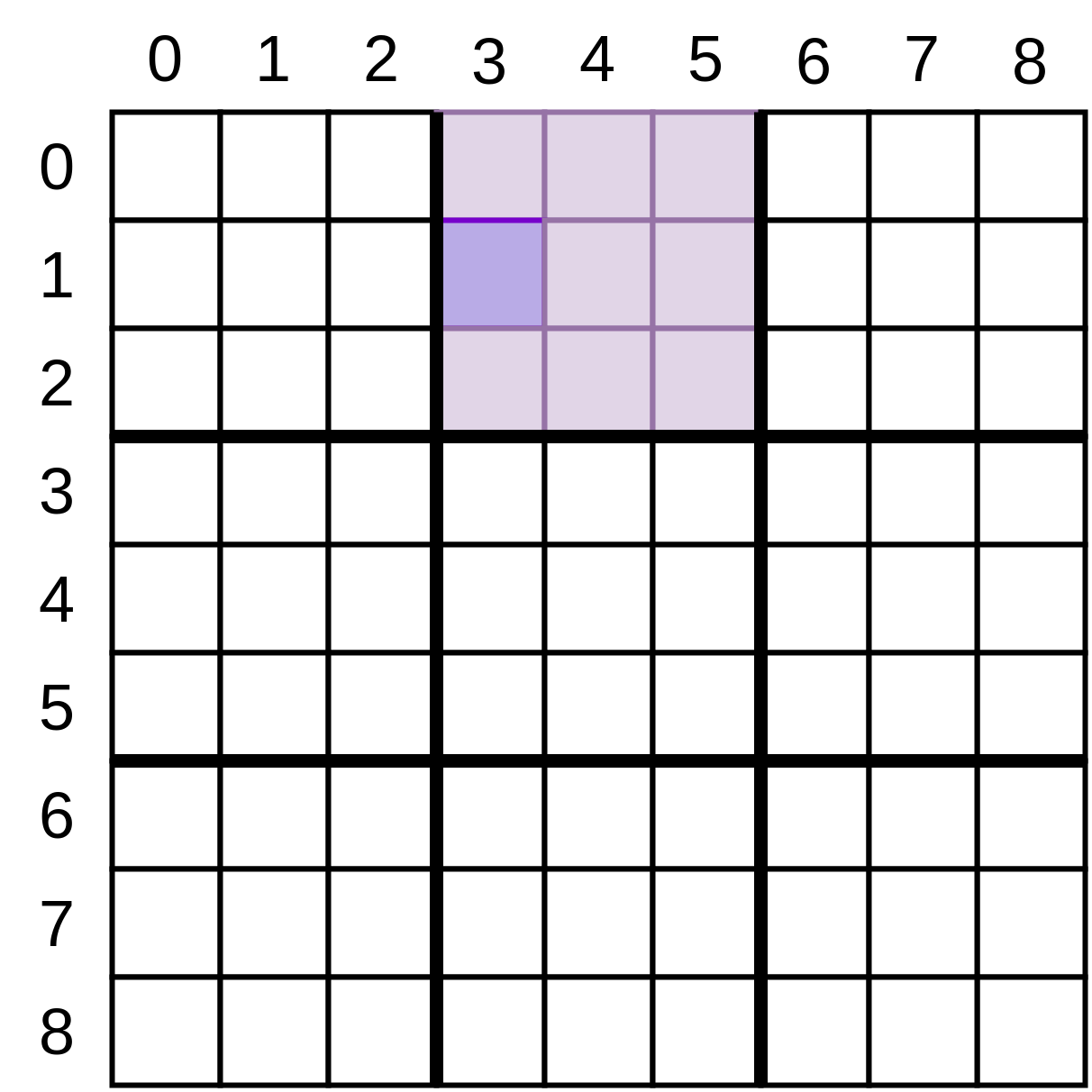
In the image above, you’re examining cell (3, 1), so your generator will produce coordinate pairs corresponding to all the lightly shaded cells, skipping the coordinates that were passed in:
(3, 0), (4, 0), (5, 0), (4, 1), (5, 1), (3, 2), (4, 2), (5, 2)
Putting the logic for determining this small square in a separate utility function keeps the flow of your other functions more readable. Making this a generator allows you to use it in a for loop to iterate through each of the values.
The function to do this involves using the limitations of integer math:
# sudokusolve.py
def small_square(x, y):
    upperX = ((x + 3) // 3) * 3
    upperY = ((y + 3) // 3) * 3
    lowerX = upperX - 3
    lowerY = upperY - 3
    for subX in range(lowerX, upperX):
        for subY in range(lowerY, upperY):
            # If subX != x or subY != y:
            if not (subX == x and subY == y):
                yield subX, subY
There are a lot of threes in a couple of those lines, which makes lines like ((x + 3) // 3) * 3 look confusing. Here’s what happens when x is 1.
>>> x = 1
>>> x + 3
4
>>> (x + 3) // 3
1
>>> ((x + 3) // 3) * 3
3
Using the rounding of integer math allows you to get the next-highest multiple of three above a given value. Once you have this, subtracting three will give you the multiple of three below the given number.
There are a few more low-level utility functions to examine before you start building on top of them.
Moving to the Next Spot
Your solution will need to walk through the grid structure one cell at a time. This means that at some point, you’ll need to figure out what the next position should be. compute_next_position() to the rescue!
compute_next_position() takes the current x- and y-coordinates as input and returns a tuple containing a finished flag along with the x- and y-coordinates of the next position:
# sudokusolve.py
def compute_next_position(x, y):
    nextY = y
    nextX = (x + 1) % 9
    if nextX < x:
        nextY = (y + 1) % 9
        if nextY < y:
            return (True, 0, 0)
    return (False, nextX, nextY)
The finished flag tells the caller that the algorithm has walked off the end of the puzzle and has completed all the squares. You’ll see how that’s used in a later section.
Removing Impossible Numbers
Your final low-level utility is quite small. It takes an integer value and an iterable. If the value is nonzero and appears in the iterable, then the function removes it from the iterable:
# sudokusolve.py
def test_and_remove(value, possible):
    if value != 0 and value in possible:
        possible.remove(value)
Typically, you wouldn’t make this small bit of functionality into a function. You’ll use this function several times, though, so it’s best to follow the DRY principle and pull it up to a function.
Now you’ve seen the bottom level of the functionality pyramid. It’s time to step up and use those tools to build a more complex function. You’re almost ready to solve the puzzle!
Finding What’s Possible
Your next function makes use of some of the low-level functions you’ve just walked through. Given a grid and a position on that grid, it determines what values that position could still have:
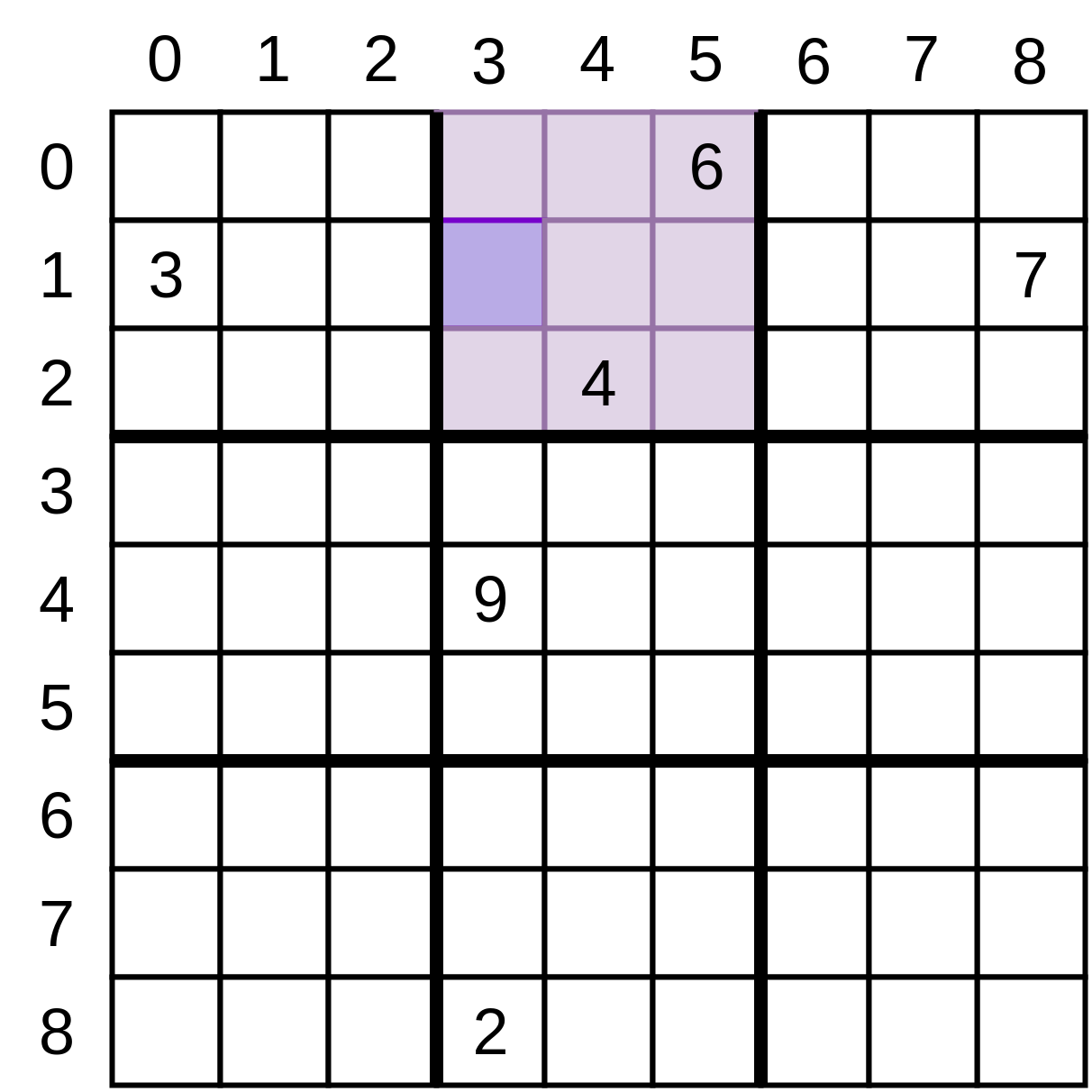
For the grid above, at the position (3, 1), the possible values are [1, 5, 8] because the other values are all present, either in that row or column or in the small square you looked at earlier.
This is the responsibility of detect_possible():
# sudokusolve.py
def detect_possible(grid, x, y):
    if grid[x][y]:
        return [grid[x][y]]

    possible = set(range(1, 10))
    # Test horizontal and vertical
    for index in range(9):
        if index != y:
            test_and_remove(grid[x][index], possible)
        if index != x:
            test_and_remove(grid[index][y], possible)

    # Test in small square
    for subX, subY in small_square(x, y):
        test_and_remove(grid[subX][subY], possible)

    return list(possible)
The function starts by checking if the given position at x and y already has a nonzero value. If so, then that’s the only possible value and it returns.
If not, then the function creates a set of the numbers one through nine. The function proceeds to check different blocking numbers and removes those from this set.
It starts by checking the column and row of the given position. This can be done with a single loop by just alternating which subscript changes. grid[x][index] checks values in the same column, while grid[index][y] checks those values in the same row. You can see that you’re using test_and_remove() here to simplify the code.
Once those values have been removed from your possible set, the function moves on to the small square. This is where the small_square() generator you created before comes in handy. You can use it to iterate over each position in the small square, again using test_and_remove() to eliminate any known values from your possible list.
Once all the known blocking values have been removed from your set, you have the list of all possible values for that position on that grid.
You might wonder why the code and its description make a point about the position being “on that grid.” In your next function, you’ll see that the program makes many copies of the grid as it tries to solve it.
Solving It
You’ve reached the heart of this solution: solve()! This function is recursive, so a little up-front explanation might help.
The general design of solve() is based on testing a single position at a time. For the position of interest, the algorithm gets the list of possible values and then selects those values, one at a time, to be in this position.
For each of these values, it creates a grid with the guessed value in this position. It then calls a function to test for a solution, passing in the new grid and the next position.
It just so happens that the function it calls is itself.
For any recursion, you need a termination condition. This algorithm has four of them:
- There are no possible values for this position. That indicates the solution it’s testing can’t work.
- It’s walked to the end of the grid and found a possible value for each position. The puzzle is solved!
- One of the guesses at this position, when passed back to the solver, returns a solution.
- It’s tried all possible values at this position and none of them will work.
Let’s look at the code for this and see how it all plays out:
# sudokusolve.py
import copy

def solve(start, x, y):
    temp = copy.deepcopy(start)
    while True:
        possible = detect_possible(temp, x, y)
        if not possible:
            return False

        finished, nextX, nextY = compute_next_position(x, y)
        if finished:
            temp[x][y] = possible[0]
            return temp

        if len(possible) > 1:
            break
        temp[x][y] = possible[0]
        x = nextX
        y = nextY

    for guess in possible:
        temp[x][y] = guess
        result = solve(temp, nextX, nextY)
        if result:
            return result
    return False
The first thing to note in this function is that it makes a .deepcopy() of the grid. It does a deep copy because the algorithm needs to keep track of exactly where it was at any point in the recursion. If the function made only a shallow copy, then every recursive version of this function would use the same grid.
Once the grid is copied, solve() can work with the new copy, temp. A position on the grid was passed in, so that’s the number that this version of the function will solve. The first step is to see what values are possible in this position. As you saw earlier, detect_possible() returns a list of possible values that may be empty.
If there are no possible values, then you’ve hit the first termination condition for the recursion. The function returns False, and the calling routine moves on.
If there are possible values, then you need to move on and see if any of them is a solution. Before you do that, you can add a little optimization to the code. If there’s only a single possible value, then you can insert that value and move on to the next position. The solution shown does this in a loop, so you can place multiple numbers into the grid without having to recur.
This may seem like a small improvement, and I’ll admit my first implementation did not include this. But some testing showed that this solution was dramatically faster than simply recurring here at the price of more complex code.
Note: This is an excellent point to bring up during an interview even if you don’t add the code to do this. Showing them that you’re thinking about trading off speed against complexity is a strong positive signal to interviewers.
Sometimes, of course, there will be multiple possible values for the current position, and you’ll need to decide if any of them will lead to a solution. Fortunately, you’ve already determined the next position in the grid, so you can forgo placing the possible values.
If the next position is off the end of the grid, then the current position is the final one to fill. If you know that there’s at least one possible value for this position, then you’ve found a solution! The current position is filled in and the completed grid is returned up to the calling function.
If the next position is still on the grid, then you loop through each possible value for the current spot, filling in the guess at the current position and then calling solve() with the temp grid and the new position to test.
solve() can return only a completed grid or False, so if any of the possible guesses returns a result that isn’t False, then a result has been found, and that grid can be returned up the stack.
If all possible guesses have been made and none of them is a solution, then the grid that was passed in is unsolvable. If this is the top-level call, then that means the puzzle is unsolvable. If the call is lower in the recursion tree, then it just means that this branch of the recursion tree isn’t viable.
Putting It All Together
At this point, you’re almost through the solution. There’s only one final function left, sudoku_solve():
# sudokusolve.py
def sudoku_solve(input_string):
    grid = line_to_grid(input_string)
    answer = solve(grid, 0, 0)
    if answer:
        return grid_to_line(answer)
    else:
        return "Unsolvable"
This function does three things:
- Converts the input string into a grid
- Calls
solve()with that grid to get a solution - Returns the solution as a string or
"Unsolvable"if there’s no solution
That’s it! You’ve walked through a solution for the sudoku solver problem.
Interview Discussion Topics
The sudoku solver solution you just walked through is a good deal of code for an interview situation. Part of an interview process would likely be to discuss some of the code and, more importantly, some of the design trade-offs you made. Let’s look at a few of those trade-offs.
Recursion
The biggest design decision revolves around using recursion. It’s possible to write a non-recursive solution to any problem that has a recursive solution. Why choose recursion over another option?
This is a discussion that depends not only on the problem but also on the developers involved in writing and maintaining the solution. Some problems lend themselves to rather clean recursive solutions, and some don’t.
In general, recursive solutions will take more time to run and use more memory than non-recursive solutions. But that’s not always true and, more importantly, it’s not always important.
Similarly, some teams of developers are comfortable with recursive solutions, while others find them exotic or unnecessarily complex. Maintainability should play into your design decisions as well.
One good discussion to have about a decision like this is around performance. How fast does this solution need to execute? Will it be used to solve billions of puzzles or just a handful? Will it run on a small embedded system with memory constraints, or will it be on a large server?
These external factors can help you decide which is a better design decision. These are great topics to bring up in an interview as you’re working through a problem or discussing code. A single product might have places where performance is critical (doing ray tracing on a graphics algorithm, for example) and places where it doesn’t matter at all (such as parsing the version number during installation).
Bringing up topics like this during an interview shows that you’re not only thinking about solving an abstract problem, but you’re also willing and able to take it to the next level and solve a specific problem facing the team.
Readability and Maintainability
Sometimes it’s worth picking a solution that’s slower in order to make a solution that’s easier to work with, debug, and extend. The decision in the sudoku solver challenge to convert the data structure to a grid is one of those decisions.
That design decision likely slows down the program, but unless you’ve measured, you don’t know. Even if it does, putting the data structure into a form that’s natural for the problem can make the code easier to comprehend.
It’s entirely possible to write a solver that operates on the linear strings you’re given as input. It’s likely faster and probably takes less memory, but small_square(), among others, will be a lot harder to write, read, and maintain in this version.
Missteps
Another thing to discuss with an interviewer, whether you’re live coding or discussing code you wrote offline, is the mistakes and false turns you took along the way.
This is a little less obvious and can be slightly detrimental, but particularly if you’re live coding, taking a step to refactor code that isn’t right or could be better can show how you work. Few developers can write perfect code the first time. Heck, few developers can write good code the first time.
Good developers write the code, then go back and refactor it and fix it. For example, my first implementation of detect_possible() looked like this:
# sudokusolve.py
def first_detect_possible(x, y, grid):
    print(f"position [{x}][{y}] = {grid[x][y]}")
    possible = set(range(1, 10))

    # Test horizontal
    for index, value in enumerate(grid[x]):
        if index != y:
            if grid[x][index] != 0:
                possible.remove(grid[x][index])
    # Test vertical
    for index, row in enumerate(grid):
        if index != x:
            if grid[index][y] != 0:
                possible.remove(grid[index][y])

    print(possible)
Ignoring that it doesn’t consider the small_square() information, this code can be improved. If you compare this to the final version of detect_possible() above, you’ll see that the final version uses a single loop to test both the horizontal and the vertical dimensions.
Wrapping Up
That’s your tour through a sudoku solver solution. There’s more information available on formats for storing puzzles and a huge list of sudoku puzzles you can test your algorithm on.
That’s the end of your Python practice problems adventure! But if you’d like more, head on over to the video course Write and Test a Python Function: Interview Practice to see an experienced developer tackle an interview problem in real time.
Conclusion
Congratulations on working through this set of Python practice problems! You’ve gotten some practice applying your Python skills and also spent some time thinking about how you can respond in different interviewing situations.
In this tutorial, you learned how to:
- Write code for interview-style problems
- Discuss your solutions during the interview
- Work through frequently overlooked details
- Talk about design decisions and trade-offs
Remember, you can download the skeleton code for these problems by clicking on the link below:
Download the sample code: Click here to get the code you’ll use to work through the Python practice problems in this tutorial.
Feel free to reach out in the comments section with any questions you have or suggestions for other Python practice problems you’d like to see! Also check out our “Ace Your Python Coding Interview” Learning Path to get more resources and for boosting your Python interview skills.
Good luck with the interview!