The Fourier transform is a powerful tool for analyzing signals and is used in everything from audio processing to image compression. SciPy provides a mature implementation in its scipy.fft module, and in this tutorial, you’ll learn how to use it.
The scipy.fft module may look intimidating at first since there are many functions, often with similar names, and the documentation uses a lot of technical terms without explanation. The good news is that you only need to understand a few core concepts to start using the module.
Don’t worry if you’re not comfortable with math! You’ll get a feel for the algorithm through concrete examples, and there will be links to further resources if you want to dive into the equations. For a visual introduction to how the Fourier transform works, you might like 3Blue1Brown’s video.
In this tutorial, you’ll learn:
- How and when to use the Fourier transform
- How to select the correct function from
scipy.fftfor your use case - How to view and modify the frequency spectrum of a signal
- Which different transforms are available in
scipy.fft
If you’d like a summary of this tutorial to keep after you finish reading, then download the cheat sheet below. It has explanations of all the functions in the scipy.fft module as well as a breakdown of the different types of transform that are available:
scipy.fft Cheat Sheet: Click here to get access to a free scipy.fft cheat sheet that summarizes the techniques explained in this tutorial.
The scipy.fft Module
The Fourier transform is a crucial tool in many applications, especially in scientific computing and data science. As such, SciPy has long provided an implementation of it and its related transforms. Initially, SciPy provided the scipy.fftpack module, but they have since updated their implementation and moved it to the scipy.fft module.
SciPy is packed full of functionality. For a more general introduction to the library, check out Scientific Python: Using SciPy for Optimization.
Install SciPy and Matplotlib
Before you can get started, you’ll need to install SciPy and Matplotlib. You can do this one of two ways:
-
Install with Anaconda: Download and install the Anaconda Individual Edition. It comes with SciPy and Matplotlib, so once you follow the steps in the installer, you’re done!
-
Install with
pip: If you already havepipinstalled, then you can install the libraries with the following command:ShellCopied!$ python -m pip install -U scipy matplotlib
You can verify the installation worked by typing python in your terminal and running the following code:
>>> import scipy, matplotlib
>>> print(scipy.__file__)
/usr/local/lib/python3.6/dist-packages/scipy/__init__.py
>>> print(matplotlib.__file__)
/usr/local/lib/python3.6/dist-packages/matplotlib/__init__.py
This code imports SciPy and Matplotlib and prints the location of the modules. Your computer will probably show different paths, but as long as it prints a path, the installation worked.
SciPy is now installed! Now it’s time to take a look at the differences between scipy.fft and scipy.fftpack.
scipy.fft vs scipy.fftpack
When looking at the SciPy documentation, you may come across two modules that look very similar:
scipy.fftscipy.fftpack
The scipy.fft module is newer and should be preferred over scipy.fftpack. You can read more about the change in the release notes for SciPy 1.4.0, but here’s a quick summary:
scipy.ffthas an improved API.scipy.fftenables using multiple workers, which can provide a speed boost in some situations.scipy.fftpackis considered legacy, and SciPy recommends usingscipy.fftinstead.
Unless you have a good reason to use scipy.fftpack, you should stick with scipy.fft.
scipy.fft vs numpy.fft
SciPy’s fast Fourier transform (FFT) implementation contains more features and is more likely to get bug fixes than NumPy’s implementation. If given a choice, you should use the SciPy implementation.
NumPy maintains an FFT implementation for backward compatibility even though the authors believe that functionality like Fourier transforms is best placed in SciPy. See the SciPy FAQ for more details.
The Fourier Transform
Fourier analysis is a field that studies how a mathematical function can be decomposed into a series of simpler trigonometric functions. The Fourier transform is a tool from this field for decomposing a function into its component frequencies.
Okay, that definition is pretty dense. For the purposes of this tutorial, the Fourier transform is a tool that allows you to take a signal and see the power of each frequency in it. Take a look at the important terms in that sentence:
- A signal is information that changes over time. For example, audio, video, and voltage traces are all examples of signals.
- A frequency is the speed at which something repeats. For example, clocks tick at a frequency of one hertz (Hz), or one repetition per second.
- Power, in this case, just means the strength of each frequency.
The following image is a visual demonstration of frequency and power on some sine waves:
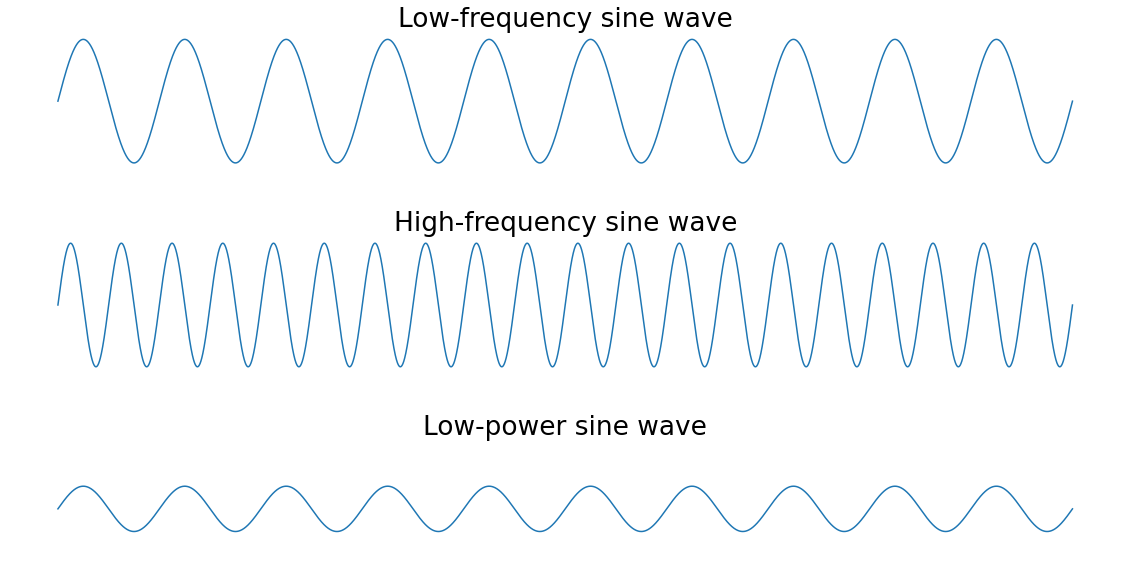
The peaks of the high-frequency sine wave are closer together than those of the low-frequency sine wave since they repeat more frequently. The low-power sine wave has smaller peaks than the other two sine waves.
To make this more concrete, imagine you used the Fourier transform on a recording of someone playing three notes on the piano at the same time. The resulting frequency spectrum would show three peaks, one for each of the notes. If the person played one note more softly than the others, then the power of that note’s frequency would be lower than the other two.
Here’s what that piano example would look like visually:
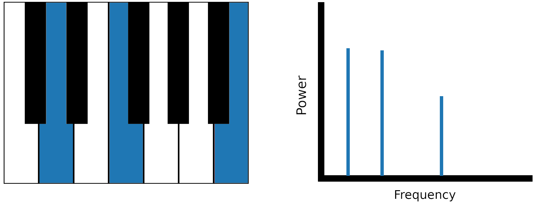
The highest note on the piano was played quieter than the other two notes, so the resulting frequency spectrum for that note has a lower peak.
Why Would You Need the Fourier Transform?
The Fourier transform is useful in many applications. For example, Shazam and other music identification services use the Fourier transform to identify songs. JPEG compression uses a variant of the Fourier transform to remove the high-frequency components of images. Speech recognition uses the Fourier transform and related transforms to recover the spoken words from raw audio.
In general, you need the Fourier transform if you need to look at the frequencies in a signal. If working with a signal in the time domain is difficult, then using the Fourier transform to move it into the frequency domain is worth trying. In the next section, you’ll look at the differences between the time and frequency domains.
Time Domain vs Frequency Domain
Throughout the rest of the tutorial, you’ll see the terms time domain and frequency domain. These two terms refer to two different ways of looking at a signal, either as its component frequencies or as information that varies over time.
In the time domain, a signal is a wave that varies in amplitude (y-axis) over time (x-axis). You’re most likely used to seeing graphs in the time domain, such as this one:

This is an image of some audio, which is a time-domain signal. The horizontal axis represents time, and the vertical axis represents amplitude.
In the frequency domain, a signal is represented as a series of frequencies (x-axis) that each have an associated power (y-axis). The following image is the above audio signal after being Fourier transformed:
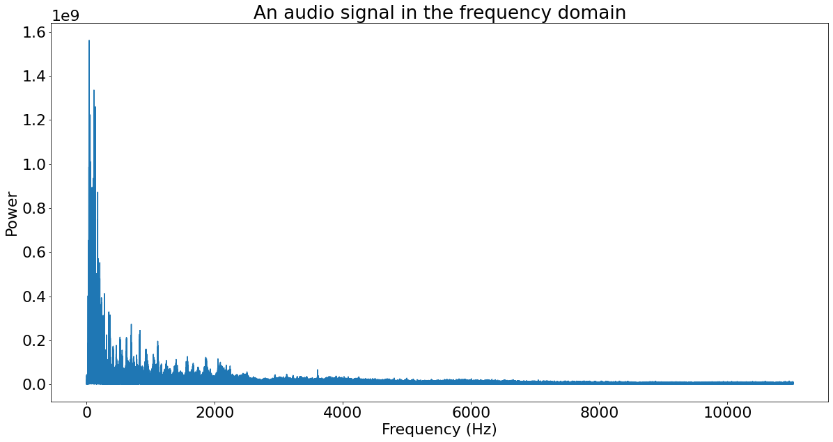
Here, the audio signal from before is represented by its constituent frequencies. Each frequency along the bottom has an associated power, producing the spectrum that you see.
For more information on the frequency domain, check out the DeepAI glossary entry.
Types of Fourier Transforms
The Fourier transform can be subdivided into different types of transform. The most basic subdivision is based on the kind of data the transform operates on: continuous functions or discrete functions. This tutorial will deal with only the discrete Fourier transform (DFT).
You’ll often see the terms DFT and FFT used interchangeably, even in this tutorial. However, they aren’t quite the same thing. The fast Fourier transform (FFT) is an algorithm for computing the discrete Fourier transform (DFT), whereas the DFT is the transform itself.
Another distinction that you’ll see made in the scipy.fft library is between different types of input. fft() accepts complex-valued input, and rfft() accepts real-valued input. Skip ahead to the section Using the Fast Fourier Transform (FFT) for an explanation of complex and real numbers.
Two other transforms are closely related to the DFT: the discrete cosine transform (DCT) and the discrete sine transform (DST). You’ll learn about those in the section The Discrete Cosine and Sine Transforms.
Practical Example: Remove Unwanted Noise From Audio
To help build your understanding of the Fourier transform and what you can do with it, you’re going to filter some audio. First, you’ll create an audio signal with a high pitched buzz in it, and then you’ll remove the buzz using the Fourier transform.
Creating a Signal
Sine waves are sometimes called pure tones because they represent a single frequency. You’ll use sine waves to generate the audio since they will form distinct peaks in the resulting frequency spectrum.
Another great thing about sine waves is that they’re straightforward to generate using NumPy. If you haven’t used NumPy before, then you can check out What Is NumPy?
Here’s some code that generates a sine wave:
import numpy as np
from matplotlib import pyplot as plt

SAMPLE_RATE = 44100  # Hertz
DURATION = 5  # Seconds

def generate_sine_wave(freq, sample_rate, duration):
    x = np.linspace(0, duration, sample_rate * duration, endpoint=False)
    frequencies = x * freq
    # 2pi because np.sin takes radians
    y = np.sin((2 * np.pi) * frequencies)
    return x, y

# Generate a 2 hertz sine wave that lasts for 5 seconds
x, y = generate_sine_wave(2, SAMPLE_RATE, DURATION)
plt.plot(x, y)
plt.show()
After you import NumPy and Matplotlib, you define two constants:
SAMPLE_RATEdetermines how many data points the signal uses to represent the sine wave per second. So if the signal had a sample rate of 10 Hz and was a five-second sine wave, then it would have10 * 5 = 50data points.DURATIONis the length of the generated sample.
Next, you define a function to generate a sine wave since you’ll use it multiple times later on. The function takes a frequency, freq, and then returns the x and y values that you’ll use to plot the wave.
The x-coordinates of the sine wave are evenly spaced between 0 and DURATION, so the code uses NumPy’s linspace() to generate them. It takes a start value, an end value, and the number of samples to generate. Setting endpoint=False is important for the Fourier transform to work properly because it assumes a signal is periodic.
np.sin() calculates the values of the sine function at each of the x-coordinates. The result is multiplied by the frequency to make the sine wave oscillate at that frequency, and the product is multiplied by 2π to convert the input values to radians.
Note: If you haven’t done much trigonometry before, or if you need a refresher, then check out Khan Academy’s trigonometry course.
After you define the function, you use it to generate a two-hertz sine wave that lasts five seconds and plot it using Matplotlib. Your sine wave plot should look something like this:
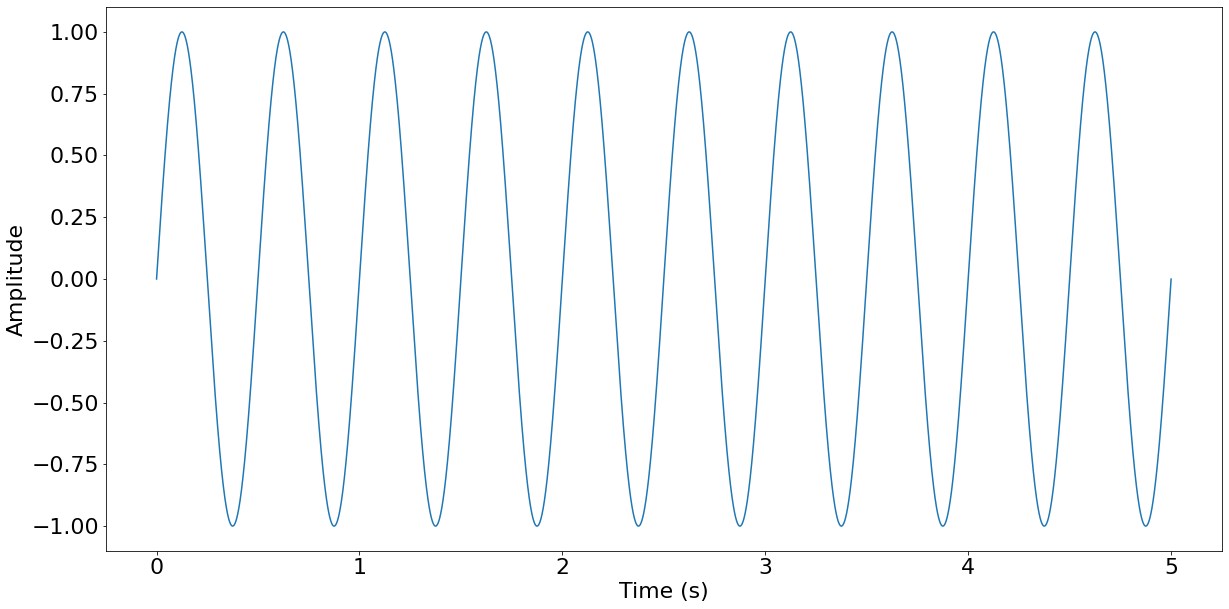
The x-axis represents time in seconds, and since there are two peaks for each second of time, you can see that the sine wave oscillates twice per second. This sine wave is too low a frequency to be audible, so in the next section, you’ll generate some higher-frequency sine waves, and you’ll see how to mix them.
Mixing Audio Signals
The good news is that mixing audio signals consists of just two steps:
- Adding the signals together
- Normalizing the result
Before you can mix the signals together, you need to generate them:
_, nice_tone = generate_sine_wave(400, SAMPLE_RATE, DURATION)
_, noise_tone = generate_sine_wave(4000, SAMPLE_RATE, DURATION)
noise_tone = noise_tone * 0.3

mixed_tone = nice_tone + noise_tone
There’s nothing new in this code example. It generates a medium-pitch tone and a high-pitch tone assigned to the variables nice_tone and noise_tone, respectively. You’ll use the high-pitch tone as your unwanted noise, so it gets multiplied by 0.3 to reduce its power. The code then adds these tones together. Note that you use the underscore (_) to discard the x values returned by generate_sine_wave().
The next step is normalization, or scaling the signal to fit into the target format. Due to how you’ll store the audio later, your target format is a 16-bit integer, which has a range from -32768 to 32767:
normalized_tone = np.int16((mixed_tone / mixed_tone.max()) * 32767)
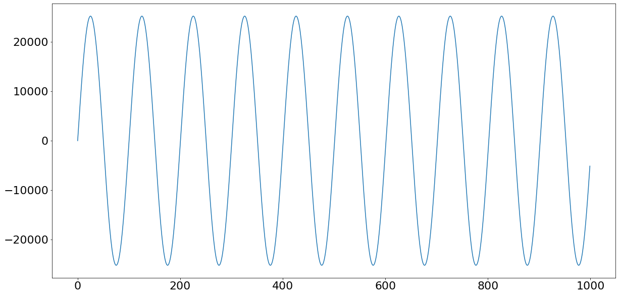
plt.plot(normalized_tone[:1000])
plt.show()
Here, the code scales mixed_tone to make it fit snugly into a 16-bit integer and then cast it to that data type using NumPy’s np.int16. Dividing mixed_tone by its maximum value scales it to between -1 and 1. When this signal is multiplied by 32767, it is scaled between -32767 and 32767, which is roughly the range of np.int16. The code plots only the first 1000 samples so you can see the structure of the signal more clearly.
Your plot should look something like this:

The signal looks like a distorted sine wave. The sine wave you see is the 400 Hz tone you generated, and the distortion is the 4000 Hz tone. If you look closely, then you can see the distortion has the shape of a sine wave.
To listen to the audio, you need to store it in a format that an audio player can read. The easiest way to do that is to use SciPy’s wavfile.write method to store it in a WAV file. 16-bit integers are a standard data type for WAV files, so you’ll normalize your signal to 16-bit integers:
from scipy.io.wavfile import write

# Remember SAMPLE_RATE = 44100 Hz is our playback rate
write("mysinewave.wav", SAMPLE_RATE, normalized_tone)
This code will write to a file mysinewave.wav in the directory where you run your Python script. You can then listen to this file using any audio player or even with Python. You’ll hear a lower tone and a higher-pitch tone. These are the 400 Hz and 4000 Hz sine waves that you mixed.
Once you’ve completed this step, you have your audio sample ready. The next step is removing the high-pitch tone using the Fourier transform!
Using the Fast Fourier Transform (FFT)
It’s time to use the FFT on your generated audio. The FFT is an algorithm that implements the Fourier transform and can calculate a frequency spectrum for a signal in the time domain, like your audio:
from scipy.fft import fft, fftfreq

# Number of samples in normalized_tone
N = SAMPLE_RATE * DURATION

yf = fft(normalized_tone)
xf = fftfreq(N, 1 / SAMPLE_RATE)

plt.plot(xf, np.abs(yf))
plt.show()
This code will calculate the Fourier transform of your generated audio and plot it. Before breaking it down, take a look at the plot that it produces:
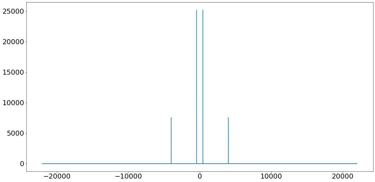
You can see two peaks in the positive frequencies and mirrors of those peaks in the negative frequencies. The positive-frequency peaks are at 400 Hz and 4000 Hz, which corresponds to the frequencies that you put into the audio.
The Fourier transform has taken your complicated, wibbly signal and turned it into just the frequencies it contains. Since you put in only two frequencies, only two frequencies have come out. The negative-positive symmetry is a side effect of putting real-valued input into the Fourier transform, but you’ll hear more about that later.
In the first couple of lines, you import the functions from scipy.fft that you’ll use later and define a variable, N, that stores the total number of samples in the signal.
After this comes the most important section, calculating the Fourier transform:
yf = fft(normalized_tone)
xf = fftfreq(N, 1 / SAMPLE_RATE)
The code calls two very important functions:
-
fft()calculates the transform itself. -
fftfreq()calculates the frequencies in the center of each bin in the output offft(). Without this, there would be no way to plot the x-axis on your frequency spectrum.
A bin is a range of values that have been grouped, like in a histogram. For more information on bins, see this Signal Processing Stack Exchange question. For the purposes of this tutorial, you can think of them as just single values.
Once you have the resulting values from the Fourier transform and their corresponding frequencies, you can plot them:
plt.plot(xf, np.abs(yf))
plt.show()
The interesting part of this code is the processing you do to yf before plotting it. You call np.abs() on yf because its values are complex.
A complex number is a number that has two parts, a real part and an imaginary part. There are many reasons why it’s useful to define numbers like this, but all you need to know right now is that they exist.
Mathematicians generally write complex numbers in the form a + bi, where a is the real part and b is the imaginary part. The i after b means that b is an imaginary number.
Note: Sometimes you’ll see complex numbers written using i, and sometimes you’ll see them written using j, such as 2 + 3i and 2 + 3j. The two are the same, but i is used more by mathematicians, and j more by engineers.
For more on complex numbers, take a look at Khan Academy’s course or the Maths is Fun page.
Since complex numbers have two parts, graphing them against frequency on a two-dimensional axis requires you to calculate a single value from them. This is where np.abs() comes in. It calculates √(a² + b²) for complex numbers, which is an overall magnitude for the two numbers together and importantly a single value.
Note: As an aside, you may have noticed that fft() returns a maximum frequency of just over 20 thousand Hertz, 22050Hz, to be exact. This value is exactly half of our sampling rate and is called the Nyquist frequency.
It’s a fundamental concept in signal processing and means that your sampling rate has to be at least twice the highest frequency in your signal.
Making It Faster With rfft()
The frequency spectrum that fft() outputted was reflected about the y-axis so that the negative half was a mirror of the positive half. This symmetry was caused by inputting real numbers (not complex numbers) to the transform.
You can use this symmetry to make your Fourier transform faster by computing only half of it. scipy.fft implements this speed hack in the form of rfft().
The great thing about rfft() is that it’s a drop-in replacement for fft(). Remember the FFT code from before:
yf = fft(normalized_tone)
xf = fftfreq(N, 1 / SAMPLE_RATE)
Swapping in rfft(), the code remains mostly the same, just with a couple of key changes:
from scipy.fft import rfft, rfftfreq

# Note the extra 'r' at the front
yf = rfft(normalized_tone)
xf = rfftfreq(N, 1 / SAMPLE_RATE)

plt.plot(xf, np.abs(yf))
plt.show()
Since rfft() returns only half the output that fft() does, it uses a different function to get the frequency mapping, rfftfreq() instead of fftfreq().
rfft() still produces complex output, so the code to plot its result remains the same. The plot, however, should look like the following since the negative frequencies will have disappeared:
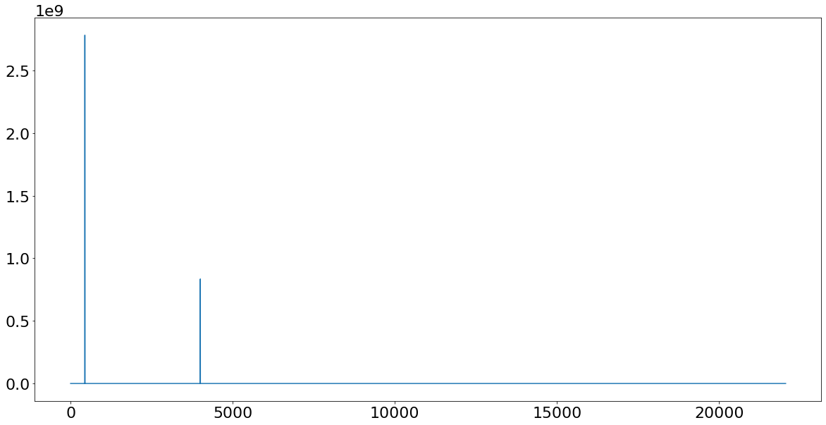
You can see that the image above is just the positive side of the frequency spectrum that fft() produces. rfft() never calculates the negative half of the frequency spectrum, which makes it faster than using fft().
Using rfft() can be up to twice as fast as using fft(), but some input lengths are faster than others. If you know you’ll be working only with real numbers, then it’s a speed hack worth knowing.
Now that you have the frequency spectrum of the signal, you can move on to filtering it.
Filtering the Signal
One great thing about the Fourier transform is that it’s reversible, so any changes you make to the signal in the frequency domain will apply when you transform it back to the time domain. You’ll take advantage of this to filter your audio and get rid of the high-pitched frequency.
Warning: The filtering technique demonstrated in this section isn’t suitable for real-world signals. See the section Avoiding Filtering Pitfalls for an explanation of why.
The values returned by rfft() represent the power of each frequency bin. If you set the power of a given bin to zero, then the frequencies in that bin will no longer be present in the resulting time-domain signal.
Using the length of xf, the maximum frequency, and the fact that the frequency bins are evenly spaced, you can work out the target frequency’s index:
# The maximum frequency is half the sample rate
points_per_freq = len(xf) / (SAMPLE_RATE / 2)

# Our target frequency is 4000 Hz
target_idx = int(points_per_freq * 4000)
You can then set yf to 0 at indices around the target frequency to get rid of it:
yf[target_idx - 1 : target_idx + 2] = 0

plt.plot(xf, np.abs(yf))
plt.show()
Your code should produce the following plot:
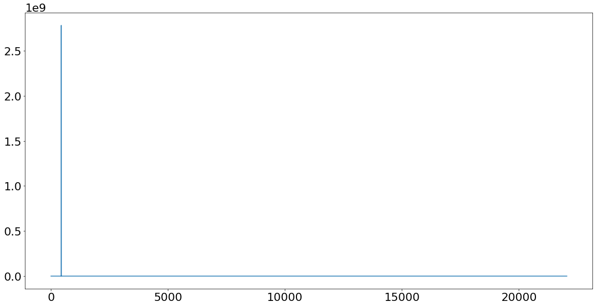
Since there’s only one peak, it looks like it worked! Next, you’ll apply the inverse Fourier transform to get back to the time domain.
Applying the Inverse FFT
Applying the inverse FFT is similar to applying the FFT:
from scipy.fft import irfft

new_sig = irfft(yf)

plt.plot(new_sig[:1000])
plt.show()
Since you are using rfft(), you need to use irfft() to apply the inverse. However, if you had used fft(), then the inverse function would have been ifft(). Your plot should now look like this:
As you can see, you now have a single sine wave oscillating at 400 Hz, and you’ve successfully removed the 4000 Hz noise.
Once again, you need to normalize the signal before writing it to a file. You can do it the same way as last time:
norm_new_sig = np.int16(new_sig * (32767 / new_sig.max()))

write("clean.wav", SAMPLE_RATE, norm_new_sig)
When you listen to this file, you’ll hear that the annoying noise has gone away!
Avoiding Filtering Pitfalls
The above example is more for educational purposes than real-world use. Replicating the process on a real-world signal, such as a piece of music, could introduce more buzz than it removes.
In the real world, you should filter signals using the filter design functions in the scipy.signal package. Filtering is a complex topic that involves a lot of math. For a good introduction, take a look at The Scientist and Engineer’s Guide to Digital Signal Processing.
The Discrete Cosine and Sine Transforms
A tutorial on the scipy.fft module wouldn’t be complete without looking at the discrete cosine transform (DCT) and the discrete sine transform (DST). These two transforms are closely related to the Fourier transform but operate entirely on real numbers. That means they take a real-valued function as an input and produce another real-valued function as an output.
SciPy implements these transforms as dct() and dst(). The i* and *n variants are the inverse and n-dimensional versions of the functions, respectively.
The DCT and DST are a bit like two halves that together make up the Fourier transform. This isn’t quite true since the math is a lot more complicated, but it’s a useful mental model.
So if the DCT and DST are like halves of a Fourier transform, then why are they useful?
For one thing, they’re faster than a full Fourier transform since they effectively do half the work. They can be even faster than rfft(). On top of this, they work entirely in real numbers, so you never have to worry about complex numbers.
Before you can learn how to choose between them, you need to understand even and odd functions. Even functions are symmetrical about the y-axis, whereas odd functions are symmetrical about the origin. To imagine this visually, take a look at the following diagrams:
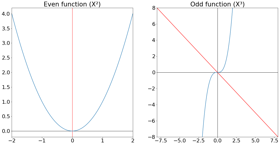
You can see that the even function is symmetrical about the y-axis. The odd function is symmetrical about y = -x, which is described as being symmetrical about the origin.
When you calculate a Fourier transform, you pretend that the function you’re calculating it on is infinite. The full Fourier transform (DFT) assumes the input function repeats itself infinitely. However, the DCT and DST assume the function is extended through symmetry. The DCT assumes the function is extended with even symmetry, and the DST assumes it’s extended with odd symmetry.
The following image illustrates how each transform imagines the function extends to infinity:
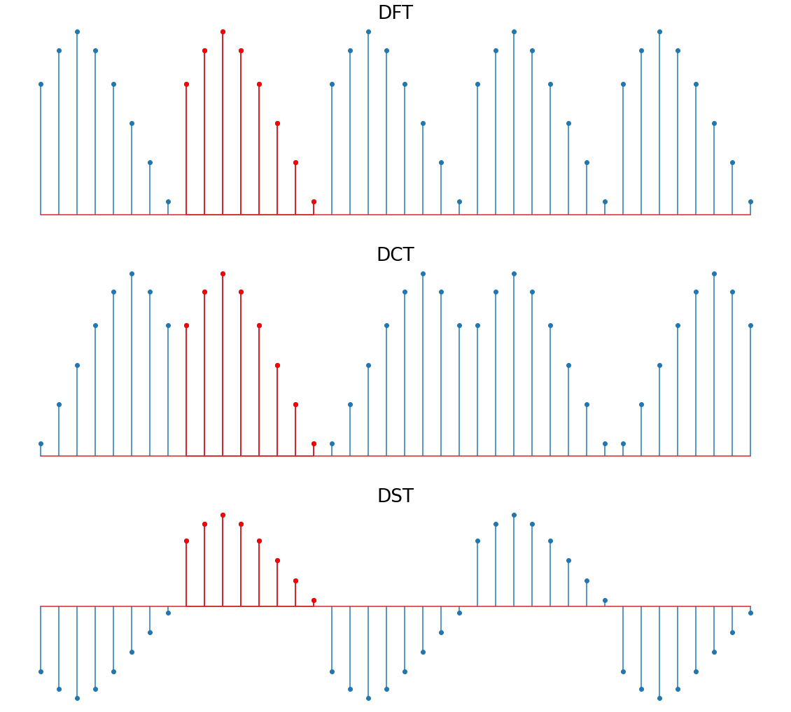
In the above image, the DFT repeats the function as is. The DCT mirrors the function vertically to extend it, and the DST mirrors it horizontally.
Note that the symmetry implied by the DST leads to big jumps in the function. These are called discontinuities and produce more high-frequency components in the resulting frequency spectrum. So unless you know your data has odd symmetry, you should use the DCT instead of the DST.
The DCT is very commonly used. There are many more examples, but the JPEG, MP3, and WebM standards all use the DCT.
Conclusion
The Fourier transform is a powerful concept that’s used in a variety of fields, from pure math to audio engineering and even finance. You’re now familiar with the discrete Fourier transform and are well equipped to apply it to filtering problems using the scipy.fft module.
In this tutorial, you learned:
- How and when to use the Fourier transform
- How to select the correct function from
scipy.fftfor your use case - What the differences are between the time domain and the frequency domain
- How to view and modify the frequency spectrum of a signal
- How using
rfft()can speed up your code
In the last section, you also learned about the discrete cosine transform and the discrete sine transform. You saw what functions to call to use them, and you learned when to use one over the other.
If you’d like a summary of this tutorial, then you can download the cheat sheet below. It has explanations of all the functions in the scipy.fft module as well as a breakdown of the different types of transform that are available:
scipy.fft Cheat Sheet: Click here to get access to a free scipy.fft cheat sheet that summarizes the techniques explained in this tutorial.
Keep exploring this fascinating topic and experimenting with transforms, and be sure to share your discoveries in the comments below!