Linear algebra is widely used across a variety of subjects, and you can use it to solve many problems once you organize the information using concepts like vectors and linear equations. In Python, most of the routines related to this subject are implemented in scipy.linalg, which offers very fast linear algebra capabilities.
In particular, linear systems play an important role in modeling a variety of real-world problems, and scipy.linalg provides tools to study and solve them in an efficient way.
In this tutorial, you’ll learn how to:
- Apply linear algebra concepts to practical problems using
scipy.linalg - Work with vectors and matrices using Python and NumPy
- Model practical problems using linear systems
- Solve linear systems using
scipy.linalg
Once you’ve gotten to know linear systems, you’ll be ready to explore matrices and least squares in the next tutorial in the series. For now, read on to get started with scipy.linalg.
Free Source Code: Click here to download the free code and dataset that you’ll use to work with linear systems and algebra in Python with scipy.linalg.
Getting Started With scipy.linalg
SciPy is an open-source Python library used for scientific computing, including several modules for common tasks in science and engineering, such as linear algebra, optimization, integration, interpolation, and signal processing. It’s part of the SciPy stack, which includes several other packages for scientific computing, such as NumPy, Matplotlib, SymPy, IPython, and pandas.
Linear algebra is a branch of mathematics that deals with linear equations and their representations using vectors and matrices. It’s a fundamental subject in several areas of engineering, and it’s a prerequisite to a deeper understanding of machine learning.
scipy.linalg includes several tools for working with linear algebra problems, including functions for performing matrix calculations, such as determinants, inverses, eigenvalues, eigenvectors, and the singular value decomposition.
In this tutorial, you’re going to use some of the functions from scipy.linalg to work on practical problems involving linear systems. In order to use scipy.linalg, you have to install and set up the SciPy library, which you can do by using the Anaconda Python distribution and the conda package and environment management system.
Note: To learn more about Anaconda and conda, check out Setting Up Python for Machine Learning on Windows.
To begin, create a conda environment and activate it:
$ conda create --name linalg
$ conda activate linalg
After you activate the conda environment, your prompt will show its name, linalg. Then you can install the necessary packages inside the environment:
(linalg) $ conda install scipy jupyter
After you execute this command, it should take a while for the system to figure out the dependencies and proceed with the installation.
Note: Besides using SciPy, you’re also going to use Jupyter Notebook to run the code in an interactive environment. Doing so isn’t mandatory, but it facilitates working with numerical and scientific applications.
For a refresher on working with Jupyter Notebooks, take a look at Jupyter Notebook: An Introduction.
If you prefer to follow along with the tutorial using a different Python distribution and the pip package manager, then expand the collapsible section below to see how to set up your environment:
First, you should create a virtual environment in which you’ll install the packages. Assuming you have Python installed, you can create and activate a virtual environment named linalg:
After you activate the virtual environment, your prompt will show its name, linalg. Then you can install the necessary packages inside the environment using pip:
(linalg) $ python -m pip install scipy jupyter
The system will take a while to figure out the dependencies and proceed with the installation. After the command finishes, you’re all set to use scipy.linalg and Jupyter.
Before opening Jupyter Notebook, you need to register the linalg environment so that you can create Notebooks using it as the kernel. To do that, with the linalg environment activated, run the following command:
(linalg) $ python -m ipykernel install --user --name linalg
Now you can open Jupyter Notebook by running the following command:
$ jupyter notebook
After Jupyter loads in your browser, create a new Notebook by clicking New → linalg, as shown below:

Inside the Notebook, you can test if the installation was successful by importing the scipy package:
In [1]: import scipy
If you don’t see an import error, then you’re ready to proceed.
Now that you’ve finished setting up the environment, you’ll see how to work with vectors and matrices in Python, which is fundamental to using scipy.linalg to work with linear algebra applications.
Working With Vectors and Matrices Using NumPy
A vector is a mathematical entity used to represent physical quantities that have both magnitude and direction. It’s a fundamental tool for solving engineering and machine learning problems. So are matrices, which are used to represent vector transformations, among other applications.
NumPy is the most used library for working with matrices and vectors in Python and is used with scipy.linalg to work with linear algebra applications. In this section, you’ll go through the basics of using it to create matrices and vectors and to perform operations on them.
To start working with matrices and vectors, the first thing you need to do in your Jupyter Notebook is to import numpy. The usual way to do it is by using the alias np:
In [1]: import numpy as np
To represent matrices and vectors, NumPy uses a special type called ndarray.
To create an ndarray object, you can use np.array(), which expects an array-like object, such as a list or a nested list.
As an example, imagine that you need to create the following matrix:

To create it with NumPy, you can use np.array(), providing a nested list containing the elements of each row of the matrix:
In [2]: A = np.array([[1, 2], [3, 4], [5, 6]])
   ...: A
Out[2]:
array([[1, 2],
       [3, 4],
       [5, 6]])
As you may notice, NumPy provides a visual representation of the matrix, in which you can identify its columns and rows.
It’s worth noting that the elements of a NumPy array must be of the same type. You can check the type of a NumPy array using .dtype:
In [3]: A.dtype
Out[3]:
dtype('int64')
Because all the elements of A are integers, the array was created with type int64. If one of the elements is a float, then the array will be created with type float64:
In [4]: A = np.array([[1.0, 2], [3, 4], [5, 6]])
   ...: A
Out[4]:
array([[1., 2.],
       [3., 4.],
       [5., 6.]])

In [5]: A.dtype
Out[5]:
dtype('float64')
To check the dimensions of an ndarray object, you can use .shape. For example, to check the dimensions of A, you can use A.shape:
In [6]: A.shape
Out[6]:
(3, 2)
As expected, the dimensions of the A matrix are 3 × 2 since A has three rows and two columns.
When working with problems involving matrices, you’ll often need to use the transpose operation, which swaps the columns and rows of a matrix.
To transpose a vector or matrix represented by an ndarray object, you can use .transpose() or .T. For example, you can obtain the transpose of A with A.T:
In [7]: A.T
Out[7]:
array([[1., 3., 5.],
       [2., 4., 6.]])
With the transposition, the columns of A become the rows of A.T, and the rows become the columns.
To create a vector, you also use np.array(), providing a list with the elements of the vector:
In [8]: v = np.array([1, 2, 3])
   ...: v
Out[8]:
array([1, 2, 3])
To check the dimensions of the vector, you use .shape just like you did before:
In [9]: v.shape
Out[9]:
(3,)
Notice that the shape of this vector is (3,) and not (3, 1) or (1, 3). This is a NumPy feature that’s relevant if you’re used to working with MATLAB. In NumPy, it’s possible to create one-dimensional arrays such as v, which may cause problems when performing operations between matrices and vectors. For example, the transposition operation has no effect on one-dimensional arrays.
Whenever you provide a one-dimensional array-like argument to np.array(), the resulting array will be a one-dimensional array. To create a two-dimensional array, you must provide a two-dimensional array-like argument, such as a nested list:
In [10]: v = np.array([[1, 2, 3]])
   ...: v.shape
Out[10]:
(1, 3)
In the above example, the dimensions of v are 1 × 3, which corresponds to the dimensions of a two-dimensional row vector. To create a column vector, you can use a nested list:
In [11]: v = np.array([[1], [2], [3]])
   ...: v.shape
Out[11]:
(3, 1)
In this case, the dimensions of v are 3 × 1, which corresponds to the dimensions of a two-dimensional column vector.
Using nested lists to create vectors can be laborious, especially for column vectors, which you’ll probably use the most. As an alternative, you can create a one-dimensional vector, providing a flat list to np.array, and use .reshape() to change the dimensions of the ndarray object:
In [12]: v = np.array([1, 2, 3]).reshape(3, 1)
   ...: v.shape
Out[12]:
(3, 1)
In the above example, you use .reshape() to obtain a column vector with the shape (3, 1) from a one-dimensional vector with the shape (3,). It’s worth noting that .reshape() expects the number of elements of the new array to be compatible with the number of elements of the original array. In other words, the number of elements in the array with the new shape must be equal to the number of elements in the original array.
In this example, you could also use .reshape() without explicitly defining the number of rows of the array:
In [13]: v = np.array([1, 2, 3]).reshape(-1, 1)
   ...: v.shape
Out[13]:
(3, 1)
Here, the -1 that you provide as an argument to .reshape() represents the number of rows necessary for the new array to have just one column, as specified by the second argument. In this case, because the original array has three elements, the number of rows for the new array will be 3.
In practical applications, you often need to create matrices of zeros, ones, or random elements. For that, NumPy provides some convenience functions, which you’ll see next.
Using Convenience Functions to Create Arrays
NumPy also provides some convenience functions to create arrays. For example, to create an array filled with zeros, you can use np.zeros():
In [1]: import numpy as np

In [2]: np.zeros((3, 2))
Out[2]:
array([[0., 0.],
       [0., 0.],
       [0., 0.]])
As its first argument, np.zeros() expects a tuple indicating the shape of the array that you want to create, and it returns an array of the type float64.
Note: To specify the type of array that np.zeros() will create, you can pass in an argument for dtype. For example, np.zeros((3, 2), dtype=int) creates an integer array.
Similarly, to create arrays filled with ones, you can use np.ones():
In [3]: np.ones((2, 3))
Out[3]:
array([[1., 1., 1.],
       [1., 1., 1.]])
It’s worth noting that np.ones() also returns an array of the type float64.
To create arrays with random elements, you can use np.random.rand():
In [4]: np.random.rand(3, 2)
Out[4]:
array([[0.8206045 , 0.54470809],
       [0.9490381 , 0.05677859],
       [0.71148476, 0.4709059 ]])
np.random.rand() returns an array with random numbers between 0 and 1, taken from a uniform distribution. Notice that, unlike np.zeros() and np.ones(), np.random.rand() doesn’t expect a tuple as its argument.
Similarly, to obtain an array with random elements taken from a normal distribution with zero mean and unit variance, you can use np.random.randn():
In [5]: np.random.randn(3, 2)
Out[5]:
array([[-1.20019512, -1.78337814],
       [-0.22135221, -0.38805899],
       [ 0.17620202, -2.05176764]])
Now that you’ve gone through creating arrays, you’ll see how to perform operations with them.
Performing Operations on NumPy Arrays
The usual Python operations using the addition (+), subtraction (-), multiplication (*), division (/), and exponent (**) operators on arrays are always performed element-wise. If one of the operands is a scalar, then you’ll perform the operation between the scalar and each element of the array.
For example, to create a matrix filled with elements equal to 10, you can use np.ones() and multiply the output by 10 using the * operator:
In [1]: import numpy as np

In [2]: 10 * np.ones((2, 2))
Out[2]:
array([[10., 10.],
       [10., 10.]])
If both operands are arrays of the same shape, then you’ll perform the operation between the corresponding elements of the arrays:
In [3]: A = 10 * np.ones((2, 2))
   ...: B = np.array([[2, 2], [5, 5]])
   ...: A * B
Out[3]:
array([[20., 20.],
       [50., 50.]])
Here, you multiply each element of matrix A by the corresponding element of matrix B.
To perform matrix multiplication according to the linear algebra rules, you can use the matrix multiplication operator (@):
In [4]: A = np.array([[1, 2], [3, 4]])
   ...: v = np.array([[5], [6]])
   ...: A @ v
Out[4]:
array([[17],
       [39]])
Here, you multiply a 2 × 2 matrix named A by a 2 × 1 vector named v.
You could obtain the same result using np.dot(), although you’re encouraged to use @ instead:
In [5]: A = np.array([[1, 2], [3, 4]])
   ...: v = np.array([[5], [6]])
   ...: np.dot(A, v)
Out[5]:
array([[17],
       [39]])
Besides offering the basic operations to work with matrices and vectors, NumPy also provides some specific functions to work with linear algebra in numpy.linalg. However, for those applications, scipy.linalg presents some advantages, as you’ll see next.
Comparing scipy.linalg With numpy.linalg
NumPy includes some tools for working with linear algebra applications in the numpy.linalg module. However, unless you don’t want to add SciPy as a dependency to your project, it’s typically better to use scipy.linalg for the following reasons:
-
As the official documentation explains,
scipy.linalgcontains all the functions innumpy.linalgplus some extra advanced functions that aren’t included innumpy.linalg. -
scipy.linalgis always compiled with support for BLAS and LAPACK, which are libraries including routines for performing numerical operations in an optimized way. Fornumpy.linalg, the use of BLAS and LAPACK is optional. Thus, depending on how you install NumPy,scipy.linalgfunctions might be faster than the ones fromnumpy.linalg.
All in all, considering that scientific and technical applications generally don’t have restrictions regarding dependencies, it’s generally a good idea to install SciPy and use scipy.linalg instead of numpy.linalg.
In the following section, you’re going to use scipy.linalg tools to work with linear systems. You’ll begin by going through the basics with a straightforward example, and then you’ll apply the concepts to a practical problem.
Using scipy.linalg.solve() to Solve Linear Systems
Linear systems can be a useful tool for finding the solution to several practical and important problems, including problems related to vehicle traffic, chemical equations, electrical circuits, and polynomial interpolation.
In this section, you’ll learn how to use scipy.linalg.solve() to solve linear systems. But before getting your hands into the code, it’s important to understand the basics.
Getting to Know Linear Systems
A linear system or, more precisely, a system of linear equations, is a set of equations linearly relating to a set of variables. Here’s an example of a linear system relating to the variables x₁, x₂, and x₃:

Here you have three equations involving three variables. In order to have a linear system, the values K₁, …, K₉ and b₁, b₂, b₃ must be constants.
When there are just two or three equations and variables, it’s feasible to perform the calculations manually, combine the equations, and find the values for the variables. However, with four or more variables, it takes a considerable amount of time to solve a linear system manually, and the risk of making mistakes increases.
Practical applications generally involve a large number of variables, which makes it infeasible to solve linear systems manually. Luckily, there are some tools that can do this hard work, such as scipy.linalg.solve().
Using scipy.linalg.solve()
SciPy provides scipy.linalg.solve() to solve linear systems quickly and reliably. To see how it works, consider the following system:

In order to use scipy.linalg.solve(), you need to first write the linear system as a matrix product, as in the following equation:

Notice that you’ll arrive at the original equations of the system after calculating the matrix product. The inputs that scipy.linalg.solve() expects are the matrix A and the vector b, which you can define using NumPy arrays. This way, you can solve the system using the following code:
 1In [1]: import numpy as np
 2   ...: from scipy import linalg
 3
 4In [2]: A = np.array(
 5   ...:    [
 6   ...:        [3, 2],
 7   ...:        [2, -1],
 8   ...:    ]
 9   ...: )
10
11In [3]: b = np.array([12, 1]).reshape((2, 1))
12
13In [4]: x = linalg.solve(A, b)
14   ...: x
15Out[4]:
16array([[2.],
17       [3.]])
Here’s a breakdown of what’s happening:
-
Lines 1 and 2 import NumPy as
np, along withlinalgfromscipy. -
Lines 4 to 9 create the coefficients matrix as a NumPy array and call it
A. -
Line 11 creates the independent terms vector using a NumPy array called
b. To make it a column vector with two lines, you use.reshape((2, 1)). -
Lines 13 and 14 call
linalg.solve()to solve the linear system characterized byAandb, with the result stored inx, which is printed. Note thatsolve()returns the solution with floating-point components, even though all the elements of the original arrays are integers.
If you replace x₁=2 and x₂=3 in the original equations, then you can verify that this is the solution to the system.
Now that you’ve gone through the basics of using scipy.linalg.solve(), it’s time to try a practical application of linear systems.
Solving a Practical Problem: Building a Meal Plan
One sort of problem that you would generally solve with linear systems is when you need to find the proportions of components needed to obtain a certain mixture. Below, you’re going to use this idea to build a meal plan, mixing different foods in order to get a balanced diet.
For that, assume that a balanced diet should include the following:
- 170 units of vitamin A
- 180 units of vitamin B
- 140 units of vitamin C
- 180 units of vitamin D
- 350 units of vitamin E
Your task is to find the quantities of each different food in order to obtain the specified amounts of the necessary vitamins. In the following table, you have the results of analyzing one gram of each food in terms of units of each vitamin:
| Food | Vitamin A | Vitamin B | Vitamin C | Vitamin D | Vitamin E |
|---|---|---|---|---|---|
| #1 | 1 | 10 | 1 | 2 | 2 |
| #2 | 9 | 1 | 0 | 1 | 1 |
| #3 | 2 | 2 | 5 | 1 | 2 |
| #4 | 1 | 1 | 1 | 2 | 13 |
| #5 | 1 | 1 | 1 | 9 | 2 |
By denoting food 1 as x₁ and so on, and considering you’re going to mix x₁ units of food 1, x₂ units of food 2, and so on, you can write an expression for the amount of vitamin A that you’d get in the combination. Considering that a balanced diet should include 170 units of vitamin A, you can use the data from the Vitamin A column to write the following equation:

Repeating the same procedure for vitamins B, C, D, and E, you arrive at the following linear system:

To use scipy.linalg.solve(), you have to obtain the coefficients matrix A and the independent terms vector b, which are given by the following:
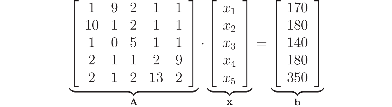
Now you can use scipy.linalg.solve() to find out the quantities x₁, …, x₅:
In [1]: import numpy as np
   ...: from scipy import linalg

In [2]: A = np.array(
   ...:     [
   ...:         [1, 9, 2, 1, 1],
   ...:         [10, 1, 2, 1, 1],
   ...:         [1, 0, 5, 1, 1],
   ...:         [2, 1, 1, 2, 9],
   ...:         [2, 1, 2, 13, 2],
   ...:     ]
   ...: )

In [3]: b = np.array([170, 180, 140, 180, 350]).reshape((5, 1))

In [4]: x = linalg.solve(A, b)
   ...: x
Out[4]:
array([[10.],
       [10.],
       [20.],
       [20.],
       [10.]])
This indicates that a balanced diet should include 10 units of food 1, 10 units of food 2, 20 units of food 3, 20 units of food 4, and 10 units of food 5.
Conclusion
Congratulations! You’ve learned how to use some linear algebra concepts and how to use scipy.linalg to solve problems involving linear systems. You’ve seen that vectors and matrices are useful for representing data and that, by using linear algebra concepts, you can model practical problems and solve them in an efficient manner.
In this tutorial, you’ve learned how to:
- Apply linear algebra concepts to practical problems using
scipy.linalg - Work with vectors and matrices using Python and NumPy
- Model practical problems using linear systems
- Solve linear systems using
scipy.linalg
Linear algebra is a very broad topic, and you can build your skill set by moving on to the next tutorial in the series, Linear Algebra in Python: Matrix Inverses and Least Squares. If you’d like to learn about some other linear algebra applications, then check out the following resources:
- Scientific Python: Using SciPy for Optimization
- Hands-On Linear Programming: Optimization With Python
- NumPy, SciPy, and Pandas: Correlation With Python
Keep studying, and feel free to leave any questions or comments below!
Free Source Code: Click here to download the free code and dataset that you’ll use to work with linear systems and algebra in Python with scipy.linalg.