
Queues are the backbone of numerous algorithms found in games, artificial intelligence, satellite navigation, and task scheduling. They’re among the top abstract data types that computer science students learn early in their education. At the same time, software engineers often leverage higher-level message queues to achieve better scalability of a microservice architecture. Plus, using queues in Python is simply fun!
Python provides a few built-in flavors of queues that you’ll see in action in this tutorial. You’re also going to get a quick primer on the theory of queues and their types. Finally, you’ll take a look at some external libraries for connecting to popular message brokers available on major cloud platform providers.
In this tutorial, you’ll learn how to:
- Differentiate between various types of queues
- Implement the queue data type in Python
- Solve practical problems by applying the right queue
- Use Python’s thread-safe, asynchronous, and interprocess queues
- Integrate Python with distributed message queue brokers through libraries
To get the most out of this tutorial, you should be familiar with Python’s sequence types, such as lists and tuples, and the higher-level collections in the standard library.
You can download the complete source code for this tutorial with the associated sample data by clicking the link in the box below:
Get Source Code: Click here to get access to the source code and sample data that you’ll use to explore queues in Python.
Learning About the Types of Queues
A queue is an abstract data type that represents a sequence of elements arranged according to a set of rules. In this section, you’ll learn about the most common types of queues and their corresponding element arrangement rules. At the very least, every queue provides operations for adding and removing elements in constant time or O(1) using the Big O notation. That means both operations should be instantaneous regardless of the queue’s size.
Some queues may support other, more specific operations. It’s time to learn more about them!
Queue: First-In, First-Out (FIFO)
The word queue can have different meanings depending on the context. However, when people refer to a queue without using any qualifiers, they usually mean a FIFO queue, which resembles a line that you might find at a grocery checkout or tourist attraction:

Note that unlike the line in the photo, where people are clustering side by side, a queue in a strict sense will be single file, with people admitted one at a time.
FIFO is short for first-in, first-out, which describes the flow of elements through the queue. Elements in such a queue will be processed on a first-come, first-served basis, which is how most real-life queues work. To better visualize the element movement in a FIFO queue, have a look at the following animation:
Notice that, at any given time, a new element is only allowed to join the queue on one end called the tail—which is on the right in this example—while the oldest element must leave the queue from the opposite end. When an element leaves the queue, then all of its followers shift by exactly one position towards the head of the queue. These few rules ensure that elements are processed in the order of their arrival.
Note: You can think of elements in a FIFO queue as cars stopping at a traffic light.
Adding an element to the FIFO queue is commonly referred to as an enqueue operation, while retrieving one from it is known as a dequeue operation. Don’t confuse a dequeue operation with the deque (double-ended queue) data type that you’ll learn about later!
Enqueuing and dequeuing are two independent operations that may be taking place at different speeds. This fact makes FIFO queues the perfect tool for buffering data in streaming scenarios and for scheduling tasks that need to wait until some shared resource becomes available. For example, a web server flooded with HTTP requests might place them in a queue instead of immediately rejecting them with an error.
Note: In programs that leverage concurrency, a FIFO queue often becomes the shared resource itself to facilitate two-way communication between asynchronous workers. By temporarily locking the read or write access to its elements, a blocking queue can elegantly coordinate a pool of producers and a pool of consumers. You’ll find more information about this use case in later sections about queues in multithreading and multiprocessing.
Another point worth noting about the queue depicted above is that it can grow without bounds as new elements arrive. Picture a checkout line stretching to the back of the store during a busy shopping season! In some situations, however, you might prefer to work with a bounded queue that has a fixed capacity known up front. A bounded queue can help to keep scarce resources under control in two ways:
- By irreversibly rejecting elements that don’t fit
- By overwriting the oldest element in the queue
Under the first strategy, once a FIFO queue becomes saturated, it won’t take any more elements until others leave the queue to make some space. You can see an animated example of how this works below:
This queue has a capacity of three, meaning it can hold at most three elements. If you try to stuff more elements into it, then they’ll bounce off into oblivion without leaving any trace behind. At the same time, as soon as the number of elements occupying the queue decreases, the queue will start accepting new elements again.
Where would you find such a bounded FIFO queue in the wild?
Most digital cameras support the burst mode for continuously shooting a series of pictures as rapidly as possible in the hope of capturing at least one sharp photo of a moving object. Because saving data onto a memory card is the bottleneck, there’s usually an internal buffer that enables the camera to keep taking new pictures while earlier ones are being compressed and saved.
In older still cameras, the buffer was usually quite small and would fill up within a few seconds. When that happened, holding the shutter button down would no longer have any effect, or the pace of snapping new pictures would reduce noticeably. The camera’s maximum speed would fully recover only after draining the data buffer.
The second strategy for dealing with incoming elements in a bounded FIFO queue lets you implement a basic cache that forgets the oldest element without considering how many times or how frequently you’ve accessed it. A FIFO cache works best when newer elements are more likely to be reused than older ones. For example, you can use the FIFO cache eviction strategy to forcefully log out users who logged in a long time ago regardless if they’re still active.
Note: For a brief comparison of other cache eviction strategies, head over to Caching in Python Using the LRU Cache Strategy.
Here’s a visual depiction of a bounded FIFO queue that can hold up to three elements but, unlike before, won’t prevent you from adding more elements:
When this queue reaches its maximum capacity, then adding a new element will first shift all existing elements by one position towards the head, discarding the oldest element and making room for the new one. Notice that the discarded element gets overwritten by its immediate neighbor.
While the unbounded FIFO queue and its two bounded counterparts cover a wide range of use cases, they all share one common feature—that is, having separate entry and exit points. In the next section, you’ll learn about yet another popular type of queue, which has a slightly different layout.
Stack: Last-In, First-Out (LIFO)
A stack is a more specialized queue, also known as a LIFO or last-in, first-out queue. It works almost exactly like a regular queue, except that elements must now join and leave it through only one end called the top of the stack. The name top reflects the fact that real-world stacks tend to be vertical. A pile of plates in the kitchen sink is an example of a stack:

When the dishwasher is full, employees will push their dirty plates on the top of the stack after having a meal. Once there are no more clean plates in the cabinet, a hungry employee will have to pop the last dirty plate from the top of the stack and clean it with a sponge before microwaving their lunch.
If there’s a much-needed fork at the bottom of the stack, then some poor soul will have to dig through all of the plates above, one by one, to get to the desired utensil. Similarly, when the cleaning personnel comes to the office at the end of a business day, they’ll have to go through the plates in reverse order before getting to the last one at the bottom of the stack.
You’ll see this element movement in the following animated stack:
Even though the LIFO queue above is oriented horizontally, it preserves the general idea of a stack. New elements grow the stack by joining it only on the right end, as in the previous examples. This time, however, only the last element pushed onto the stack can leave it. The rest must wait until there are no more elements that have joined the stack later.
Stacks are widely used in computing for various purposes. Perhaps the most familiar context for a programmer is the call stack containing the functions in the order they were called. Python will reveal this stack to you through a traceback in case of an unhandled exception. It’s usually a bounded stack with a limited capacity, which you’ll find out about during a stack overflow error caused by too many recursive calls.
In compiled languages with static type checking, local variables are allocated on the stack, which is a fast memory region. Stacks can help detect unmatched brackets in a code block or evaluate arithmetic expressions represented in reverse Polish notation (RPN). You can also use stacks to solve the Tower of Hanoi puzzle or keep track of the visited nodes in a graph or a tree traversed with the depth-first search (DFS) algorithm.
Note: When you replace the stack, or LIFO queue, with a FIFO queue in the DFS algorithm and make a few minor tweaks, then you’ll get the breadth-first search (BFS) algorithm almost for free! You’ll explore both algorithms in more detail later in this tutorial.
While a stack is a specialization of a queue, the deque or double-ended queue is a generalization that you can use as a basis to implement both FIFO and LIFO queues. You’ll see how deques work and where you can use them in the next section.
Deque: Double-Ended Queue
A double-ended queue or deque (pronounced deck) is a more generic data type that combines and extends the ideas behind the stack and the queue. It allows you to enqueue or dequeue elements from both ends in constant time at any given moment. Therefore, a deque can work as a FIFO or a LIFO queue, as well as anything in between and beyond.
Using the same example of a line of people as before, you can take advantage of a deque to model more sophisticated corner cases. In real life, the last person in the queue might get impatient and decide to leave the queue early or join another queue at a new checkout that has just opened. Conversely, someone who has booked a visit online for a particular date and time in advance may be allowed to join the queue at the front without waiting.
Below is an animation that shows an unbounded deque in action:
In this particular example, most elements generally follow one direction by joining the queue on the right and leaving it on the left, just like in a plain FIFO queue. However, some privileged elements are allowed to join the queue from the left end, while the last element can leave the queue through the opposite end.
Adding an element to a bounded deque that has already reached its full capacity will overwrite the element currently located at the opposite end. That feature might be handy for isolating the first few or the last few elements from a sequence. You may also want to stop anywhere in that sequence and then move to the left or right in smaller steps:
Suppose you were calculating the moving average of pixel intensities in a scan line of a raster image. Moving left or right would give you a preview of the few consecutive pixel values and dynamically calculate their average. This is more or less how convolution kernels work for applying filters in advanced image processing.
Most deques support two additional operations called rotate left and rotate right, which shift the elements a specified number of places in one or the other direction in a circular fashion. Because the deque’s size remains unchanged, elements that would stick out get wrapped around at the ends, as in an analog car odometer:
When rotated right, the last element in the deque becomes first. On the other hand, when rotated left, the first element becomes the last one. Perhaps you could imagine this process more easily by arranging the deque’s elements in a circle so that both ends meet. Then, rotating right and left would correspond to a clockwise and counterclockwise rotation, respectively.
Rotations, combined with the deque’s core capabilities, open up interesting possibilities. For example, you could use a deque to implement a load balancer or a task scheduler working in a round-robin fashion. In a GUI application, you could use a deque to store recently opened files, allow a user to undo and redo their actions, or let the user navigate back and forth through their web browsing history.
As you can see, deques find many practical uses, especially in tracking the most recent activity. However, some problems will require you to take advantage of yet another type of queue, which you’ll read about next.
Priority Queue: Sorted From High to Low
A priority queue is different from those you’ve seen so far because it can’t store ordinary elements. Instead, each element must now have an associated priority to compare against other elements. The queue will maintain a sorted order, letting new elements join where necessary while shuffling the existing elements around if needed. When two elements are of equal priority, they’ll follow their insertion order.
Note: Make sure to choose a data type for your priorities whose values are comparable through the comparison operators, such as less than (<). For example, integers and timestamps would be fine, while complex numbers wouldn’t work for indicating priority because they don’t implement any relevant comparison operator.
This kind of queue works in a way that’s analogous to priority boarding on a plane:

Regular passengers will join the queue at the very end unless they’re accompanied by small children, have disabilities, or have earned loyalty points, in which case they’ll be fast-tracked to the front of the line. Business-class travelers usually enjoy the luxury of a separate, much smaller queue, but even they sometimes have to let the first-class travelers pass.
The animation below illustrates a sample flow of elements having three distinct priorities through an unbounded priority queue:
Blue squares represent the lowest priority, yellow triangles are higher in the hierarchy, and red circles are the most important. A new element gets inserted between one with a higher or equal priority and another one with a lower priority. This rule resembles the insertion sort algorithm, which happens to be stable, as elements with the same priority never swap their initial places.
You could use the priority queue to sort a sequence of elements by a given key or get the top few elements. However, that would be overkill because there are far more efficient sorting algorithms available. The priority queue is better suited for situations when elements can come and go dynamically. One such situation would be searching for the shortest path in a weighted graph using Dijkstra’s algorithm, which you’ll read about later.
Note: Even though the priority queue is conceptually a sequence, its most efficient implementation builds on top of the heap data structure, which is a kind of binary tree. Therefore, the terms heap and priority queue are sometimes used interchangeably.
That was a longish introduction to the theory and taxonomy of queues. Along the way, you’ve learned about FIFO queues, stacks (LIFO queues), deques, and priority queues. You’ve also seen the difference between bounded and unbounded queues, and you’ve gotten an idea about their potential applications. Now, it’s time to take a stab at implementing some of those queues yourself.
Implementing Queues in Python
First of all, should you implement a queue yourself in Python? In most cases, the answer to that question will be a decisive no. The language comes with batteries included, and queues are no exception. In fact, you’ll discover that Python has an abundance of queue implementations suited to solving various problems.
That being said, trying to build something from scratch can be an invaluable learning experience. You might also get asked to provide a queue implementation during a technical interview. So, if you find this topic interesting, then please read on. Otherwise, if you only seek to use queues in practice, then feel free to skip this section entirely.
Representing FIFO and LIFO Queues With a Deque
To represent a FIFO queue in the computer’s memory, you’ll need a sequence that has O(1), or constant time, performance for the enqueue operation on one end, and a similarly efficient dequeue operation on the other end. As you already know by now, a deque or double-ended queue satisfies those requirements. Plus, it’s universal enough to adapt for a LIFO queue as well.
However, because coding one would be out of scope of this tutorial, you’re going to leverage Python’s deque collection from the standard library.
Note: A deque is an abstract data type that you may implement in a few ways. Using a doubly linked list as the underlying implementation will ensure that accessing and removing elements from both ends will have the desired O(1) time complexity. If your deque has a fixed size, then you can use a circular buffer instead, letting you access any element in constant time. Unlike a linked list, a circular buffer is a random-access data structure.
Why not use a Python list instead of collections.deque as a building block for your FIFO queue?
Both sequences allow for enqueuing elements with their .append() methods rather cheaply, with a small reservation for lists, which will occasionally require copying all elements to a new memory location when their number exceeds a certain threshold.
Unfortunately, dequeuing an element from the front of a list with list.pop(0), or equivalently inserting one with list.insert(0, element), is far less efficient. Such operations always shift the remaining elements, resulting in a linear, or O(n), time complexity. In contrast, deque.popleft() and deque.appendleft() avoid that step altogether.
With that, you can proceed to define your custom Queue class based on Python’s deque collection.
Building a Queue Data Type
Now that you’ve chosen a suitable queue representation, you can fire up your favorite code editor, such as Visual Studio Code or PyCharm, and create a new Python module for the different queue implementations. You can call the file queues.py (plural form) to avoid a conflict with the similarly named queue (singular form) module already available in Python’s standard library.
Note: You’ll have a closer look at the built-in queue module in a later section devoted to thread-safe queues in Python.
Because you want your custom FIFO queue to support at least the enqueue and dequeue operations, go ahead and write a bare-bones Queue class that’ll delegate those two operations to deque.append() and deque.popleft() methods, respectively:
# queues.py

from collections import deque

class Queue:
    def __init__(self):
        self._elements = deque()

    def enqueue(self, element):
        self._elements.append(element)

    def dequeue(self):
        return self._elements.popleft()
This class merely wraps a collections.deque instance and calls it ._elements. The leading underscore in the attribute’s name indicates an internal bit of implementation, which only the class should access and modify. Such fields are sometimes called private because they’re not supposed to be visible outside of the class body.
You can test your FIFO queue by importing it from the local module within an interactive Python interpreter session:
>>> from queues import Queue

>>> fifo = Queue()
>>> fifo.enqueue("1st")
>>> fifo.enqueue("2nd")
>>> fifo.enqueue("3rd")

>>> fifo.dequeue()
'1st'
>>> fifo.dequeue()
'2nd'
>>> fifo.dequeue()
'3rd'
As expected, the enqueued elements come back to you in their original order. If you want, you may improve your class by making it iterable and able to report its length and optionally accept initial elements:
# queues.py

from collections import deque

class Queue:
    def __init__(self, *elements):
        self._elements = deque(elements)

    def __len__(self):
        return len(self._elements)

    def __iter__(self):
        while len(self) > 0:
            yield self.dequeue()

    def enqueue(self, element):
        self._elements.append(element)

    def dequeue(self):
        return self._elements.popleft()
A deque takes an optional iterable, which you can provide through a varying number of positional arguments, *elements, in your initializer method. By implementing the special .__iter__() method, you’ll make your class instances usable in a for loop, while implementing .__len__() will make them compatible with the len() function. The .__iter__() method above is an example of a generator iterator, which yields elements lazily.
Note: The implementation of .__iter__() causes your custom queue to reduce its size by dequeuing elements from itself as you iterate over it.
Restart the Python interpreter and import your class again to see the updated code in action:
>>> from queues import Queue

>>> fifo = Queue("1st", "2nd", "3rd")
>>> len(fifo)
3

>>> for element in fifo:
...     print(element)
...
1st
2nd
3rd

>>> len(fifo)
0
The queue has three elements initially, but its length drops to zero after consuming all elements in a loop. Next up, you’ll implement a stack data type that’ll dequeue elements in reverse order.
Building a Stack Data Type
Building a stack data type is considerably more straightforward because you’ve already done the bulk of the hard work. Since most of the implementation will remain the same, you can extend your Queue class using inheritance and override the .dequeue() method to remove elements from the top of the stack:
# queues.py

# ...

class Stack(Queue):
    def dequeue(self):
        return self._elements.pop()
That’s it! Elements are now popped from the same end of the queue that you pushed them through before. You can quickly verify this in an interactive Python session:
>>> from queues import Stack

>>> lifo = Stack("1st", "2nd", "3rd")
>>> for element in lifo:
...     print(element)
...
3rd
2nd
1st
With an identical setup and test data as before, the elements return to you in reverse order, which is the expected behavior of a LIFO queue.
Note: In this tutorial, you use inheritance as a convenient mechanism to reuse code. However, the current class relationship isn’t semantically correct, because a stack isn’t a subtype of a queue. You could just as well define the stack first and let the queue extend it. In the real world, you should probably make both classes inherit from an abstract base class because they share the same interface.
In one-off scripts, you could probably get away with using a plain old Python list as a rudimentary stack when you don’t mind the extra overhead of having to copy the values from time to time:
>>> lifo = []

>>> lifo.append("1st")
>>> lifo.append("2nd")
>>> lifo.append("3rd")

>>> lifo.pop()
'3rd'
>>> lifo.pop()
'2nd'
>>> lifo.pop()
'1st'
Python lists are iterable out of the box. They can report their length and have a sensible textual representation. In the next section, you’ll choose them as the foundation for a priority queue.
Representing Priority Queues With a Heap
The last queue that you’ll implement in this tutorial will be a priority queue. Unlike a stack, the priority queue can’t extend the Queue class defined earlier, because it doesn’t belong to the same type hierarchy. The order of elements in a FIFO or LIFO queue is determined solely by the elements’ time of arrival. In a priority queue, it’s an element’s priority and the insertion order that together determine the ultimate position within the queue.
There are many ways to implement a priority queue, such as:
- An unordered list of elements and their priorities, which you search through every time before dequeuing the element with the highest priority
- An ordered list of elements and their priorities, which you sort every time you enqueue a new element
- An ordered list of elements and their priorities, which you keep sorted by finding the right spot for a new element using binary search
- A binary tree that maintains the heap invariant after the enqueue and dequeue operations
You can think of a priority queue as a list that needs to be sorted every time a new element arrives so that you’ll be able to remove the last one with the highest priority when performing the dequeue operation. Alternatively, you could ignore the element order until removing one with the highest priority, which you could find using the linear search algorithm.
Looking up an element in an unordered list has O(n) time complexity. Sorting the entire queue would be even more expensive, especially when exercised often. Python’s list.sort() method employs an algorithm called Timsort, which has O(n log(n)) worst-case time complexity. Inserting an element with bisect.insort() is slightly better because it can take advantage of an already sorted list, but the gain is offset by the slow insertion that follows.
Fortunately, you can be smart about keeping the elements sorted in a priority queue by using a heap data structure under the hood. It provides a more efficient implementation than those listed earlier. Here’s a table with a quick comparison of the time complexity for the enqueue and dequeue operations provided by those different implementations:
| Implementation | Enqueue | Dequeue |
|---|---|---|
| Find Max on Dequeue | O(1) | O(n) |
| Sort on Enqueue | O(n log(n)) | O(1) |
| Bisect and Insert on Enqueue | O(n) | O(1) |
| Push onto a Heap on Enqueue | O(log(n)) | O(log(n)) |
The heap has the best overall performance for large data volumes. Although using the bisection method to find the right spot for a new element is O(log(n)), the actual insertion of that element is O(n), making it less desirable than a heap.
Python has the heapq module, which conveniently provides a few functions that can turn a regular list into a heap and manipulate it efficiently. The two functions that’ll help you build a priority queue are:
heapq.heappush()heapq.heappop()
When you push a new element onto a non-empty heap, it’ll end up in the right spot, maintaining the heap invariant. Note that this doesn’t necessarily mean that the resulting elements will become sorted:
>>> from heapq import heappush

>>> fruits = []
>>> heappush(fruits, "orange")
>>> heappush(fruits, "apple")
>>> heappush(fruits, "banana")

>>> fruits
['apple', 'orange', 'banana']
Fruit names in the resulting heap in the example above don’t follow alphabetical order. If you pushed them in a different order, though, they could!
The point of a heap isn’t so much about sorting elements but rather keeping them in a certain relationship to allow for quick lookup. What really matters is that the first element on a heap always has the smallest (min-heap) or the highest (max-heap) value, depending on how you define the condition for the mentioned relationship. Python’s heaps are min-heaps, which means that the first element has the smallest value.
When you pop an element from a heap, you’ll always get the first one, while the remaining elements might shuffle a little bit:
>>> from heapq import heappop

>>> heappop(fruits)
'apple'

>>> fruits
['banana', 'orange']
Notice how the banana and orange swapped places to ensure the first element continues to be the smallest. When you tell Python to compare two string objects by value, it starts looking at their characters pairwise from left to right and checks each pair one by one. The character with a lower Unicode code point is considered smaller, which resolves the word order.
Now, how do you throw priorities into the mix? The heap compares elements by value rather than by their priority, after all. To work around this, you can leverage Python’s tuple comparison, which takes into account the tuple’s components, looking from left to right until the outcome is known:
>>> person1 = ("John", "Brown", 42)
>>> person2 = ("John", "Doe", 42)
>>> person3 = ("John", "Doe", 24)

>>> person1 < person2
True
>>> person2 < person3
False
Here, you have three tuples representing different people. Each has a first name, last name, and age. Python determines that person1 should go before person2 based on their last names since they share the same first name, but Python doesn’t look at their ages because the ordering is already known. The age becomes important in the second comparison between person2 and person3, who happen to have the same first and last names.
You can enforce a prioritized order on the heap by storing tuples whose first element is a priority. However, there will be a few fine details that you need to be careful about. You’ll learn more about them in the next section.
Building a Priority Queue Data Type
Imagine you were building software for an automotive company. Modern vehicles are practically computers on wheels, which leverage a controller area network (CAN) bus to broadcast messages about various events going on in your car, such as unlocking the doors or inflating an airbag. Clearly, some of those events are more important than others and should be prioritized accordingly.
Fun Fact: You can download a mobile app for your smartphone, such as Torque, that’ll let you connect to the CAN bus of your car over Bluetooth or an ad hoc WiFi network through a small scanner device hooked up to your car’s on-board diagnostics (OBD) port.
This setup will allow you to monitor your vehicle’s parameters in real time, even if they’re not exposed on the dashboard! This includes things like coolant temperature, battery voltage, miles per gallon, and emissions. Moreover, you’ll be able to check if your car’s ECUs report any fault codes.
It’s okay to miss a faulty headlight message or wait a little longer for the audio volume level to go down. However, when you press the brake pedal, you expect it to have an immediate effect because it’s a safety-critical subsystem. Each message has a priority in the CAN bus protocol, which tells the intermediate units whether they should relay the message further or disregard it completely.
Even though this is an oversimplification of the problem, you can think of the CAN bus as a priority queue that sorts the messages according to their importance. Now, return to your code editor and define the following class in the Python module that you created before:
# queues.py

from collections import deque
from heapq import heappop, heappush

# ...

class PriorityQueue:
    def __init__(self):
        self._elements = []

    def enqueue_with_priority(self, priority, value):
        heappush(self._elements, (priority, value))

    def dequeue(self):
        return heappop(self._elements)
It’s a basic priority queue implementation, which defines a heap of elements using a Python list and two methods that manipulate it. The .enqueue_with_priority() method takes two arguments, a priority and a corresponding value, which it then wraps in a tuple and pushes onto the heap using the heapq module. Notice that the priority comes before the value to take advantage of how Python compares tuples.
Unfortunately, there are a few problems with the above implementation that become apparent when you try to use it:
>>> from queues import PriorityQueue

>>> CRITICAL = 3
>>> IMPORTANT = 2
>>> NEUTRAL = 1

>>> messages = PriorityQueue()
>>> messages.enqueue_with_priority(IMPORTANT, "Windshield wipers turned on")
>>> messages.enqueue_with_priority(NEUTRAL, "Radio station tuned in")
>>> messages.enqueue_with_priority(CRITICAL, "Brake pedal depressed")
>>> messages.enqueue_with_priority(IMPORTANT, "Hazard lights turned on")

>>> messages.dequeue()
(1, 'Radio station tuned in')
You defined three priority levels: critical, important, and neutral. Next, you instantiated a priority queue and used it to enqueue a few messages with those priorities. However, instead of dequeuing the message with the highest priority, you got a tuple corresponding to the message with the lowest priority.
Note: Ultimately, it’s up to you how you want to define the order of your priorities. In this tutorial, a lower priority corresponds to a lower numeric value, while a higher priority has a greater value.
That said, it can be more convenient to reverse this order in some cases. For example, in Dijkstra’s shortest path algorithm, you’ll want to prioritize paths with a smaller total cost over those with a high cost. To handle such a situation, you’ll implement another class later.
Because Python’s heap is a min-heap, its first element always has the lowest value. To fix this, you can flip the sign of a priority when pushing a tuple onto the heap, making the priority a negative number so that the highest one becomes the lowest:
# queues.py

# ...

class PriorityQueue:
    def __init__(self):
        self._elements = []

    def enqueue_with_priority(self, priority, value):
        heappush(self._elements, (-priority, value))

    def dequeue(self):
        return heappop(self._elements)[1]
With this small change, you’ll push critical messages ahead of important and neutral ones. Additionally, when performing a dequeue operation, you’ll unpack the value from the tuple by accessing its second component, located at index one using the square bracket ([]) syntax.
Now, if you head back to your interactive Python interpreter, import the updated code, and enqueue the same messages once again, then they’ll come back to you in a more sensible order:
>>> messages.dequeue()
'Brake pedal depressed'

>>> messages.dequeue()
'Hazard lights turned on'

>>> messages.dequeue()
'Windshield wipers turned on'

>>> messages.dequeue()
'Radio station tuned in'
You get the critical message first, followed by the two important ones, and then the neutral message. So far, so good, right? However, there are two problems with your implementation. One of them you can already see in the output, while the other will only manifest itself under specific circumstances. Can you spot these problems?
Handling Corner Cases in Your Priority Queue
Your queue can correctly order elements by priority, but at the same time, it violates sort stability when comparing elements with equal priorities. This means that in the example above, flashing the hazard lights takes precedence over engaging the windshield wipers, even though this ordering doesn’t follow the chronology of events. Both messages have the same priority, important, so the queue should sort them by their insertion order.
To be clear, this is a direct consequence of tuple comparison in Python, which moves to the next component in a tuple if the earlier ones didn’t resolve the comparison. So, if two messages have equal priorities, then Python will compare them by value, which would be a string in your example. Strings follow the lexicographic order, in which the word Hazard comes before the word Windshield, hence the inconsistent order.
There’s another problem related to that, which would completely break the tuple comparison in rare cases. Specifically, it’d fail if you tried to enqueue an element that doesn’t support any comparison operators, such as an instance of a custom class, and the queue already contained at least one element with the same priority that you wanted to use. Consider the following data class to represent messages in your queue:
>>> from dataclasses import dataclass

>>> @dataclass
... class Message:
...     event: str
...

>>> wipers = Message("Windshield wipers turned on")
>>> hazard_lights = Message("Hazard lights turned on")

>>> wipers < hazard_lights
Traceback (most recent call last):
  ...
TypeError: '<' not supported between instances of 'Message' and 'Message'
Message objects might be more convenient to work with than plain strings, but unlike strings, they aren’t comparable unless you tell Python how to perform the comparison. As you can see, custom class instances don’t provide the implementation for the less than (<) operator by default.
As long as you enqueue messages with different priorities, Python won’t compare them by value:
>>> messages = PriorityQueue()
>>> messages.enqueue_with_priority(CRITICAL, wipers)
>>> messages.enqueue_with_priority(IMPORTANT, hazard_lights)
For example, when you enqueue a critical message and an important message, Python determines their order unambiguously by looking at the corresponding priorities. However, as soon as you try enqueuing another critical message, you’ll get a familiar error:
>>> messages.enqueue_with_priority(CRITICAL, Message("ABS engaged"))
Traceback (most recent call last):
  ...
TypeError: '<' not supported between instances of 'Message' and 'Message'
This time around, the comparison fails because two of the messages are of equal priority and Python falls back to comparing them by value, which you haven’t defined for your custom Message class instances.
You can solve both problems—that is, the sort instability and the broken tuple comparison—by introducing another component to the elements stored on the heap. This extra component should be comparable and represent the time of arrival. When placed between the element’s priority and value in a tuple, it’ll resolve the order if two elements have the same priority, regardless of their values.
The most straightforward way of representing the arrival time in a priority queue is perhaps a monotonically increasing counter. In other words, you want to count the number of enqueue operations performed without considering the potential dequeue operations that might be taking place. Then, you’ll store the current value of the counter in every enqueued element to reflect the state of your queue at that instant.
You can use the count() iterator from the itertools module to count from zero to infinity in a concise way:
# queues.py

from collections import deque
from heapq import heappop, heappush
from itertools import count

# ...

class PriorityQueue:
    def __init__(self):
        self._elements = []
        self._counter = count()

    def enqueue_with_priority(self, priority, value):
        element = (-priority, next(self._counter), value)
        heappush(self._elements, element)

    def dequeue(self):
        return heappop(self._elements)[-1]
The counter gets initialized when you create a new PriorityQueue instance. Whenever you enqueue a value, the counter increments and retains its current state in a tuple pushed onto the heap. So, if you enqueue another value with the same priority later, then the earlier one will take precedence because you enqueued it with a smaller counter.
The last tiny detail to keep in mind after introducing this extra counter component into the tuple is updating the popped value index during a dequeue operation. Because elements are tuples with three components now, you ought to return the value located at index two instead of one. However, it’d be safer to use the negative one as an index to indicate the last component of the tuple, regardless of its length.
Your priority queue is almost ready, but it’s missing the two special methods, .__len__() and .__iter__(), which you implemented in the other two queue classes. While you can’t reuse their code through inheritance, as the priority queue is not a subtype of the FIFO queue, Python provides a powerful mechanism that lets you work around that issue.
Refactoring the Code Using a Mixin Class
To reuse code across unrelated classes, you can identify their least common denominator and then extract that code into a mixin class. A mixin class is like a spice. It can’t stand on its own, so you wouldn’t typically instantiate it, but it can add that extra flavor once you mix it into another class. Here’s how it would work in practice:
# queues.py

# ...

class IterableMixin:
    def __len__(self):
        return len(self._elements)

    def __iter__(self):
        while len(self) > 0:
            yield self.dequeue()

class Queue(IterableMixin):
    # ...

class Stack(Queue):
    # ...

class PriorityQueue(IterableMixin):
    # ...
You moved the .__len__() and .__iter__() methods from the Queue class to a separate IterableMixin class and made the former extend that mixin. You also made the PriorityQueue inherit from the same mixin class. How is this different from the standard inheritance?
Unlike programming languages like Scala that support mixins directly with traits, Python uses multiple inheritance to implement the same concept. However, extending a mixin class is semantically different from extending a regular class, which is no longer a form of type specialization. To emphasize this difference, some people call it the inclusion of a mixin class rather than pure inheritance.
Notice that your mixin class refers to an ._elements attribute, which you haven’t defined yet! It’s provided by the concrete classes, such as Queue and PriorityQueue, that you throw into the mix much later. Mixins are great for encapsulating behavior rather than state, much like default methods in Java interfaces. By composing a class with one or more mixins, you can change or augment its original behavior.
Expand the collapsible section below to reveal the complete source code:
# queues.py

from collections import deque
from heapq import heappop, heappush
from itertools import count

class IterableMixin:
    def __len__(self):
        return len(self._elements)

    def __iter__(self):
        while len(self) > 0:
            yield self.dequeue()

class Queue(IterableMixin):
    def __init__(self, *elements):
        self._elements = deque(elements)

    def enqueue(self, element):
        self._elements.append(element)

    def dequeue(self):
        return self._elements.popleft()

class Stack(Queue):
    def dequeue(self):
        return self._elements.pop()

class PriorityQueue(IterableMixin):
    def __init__(self):
        self._elements = []
        self._counter = count()

    def enqueue_with_priority(self, priority, value):
        element = (-priority, next(self._counter), value)
        heappush(self._elements, element)

    def dequeue(self):
        return heappop(self._elements)[-1]
With the three queue classes in place, you can finally apply them to solving a real problem!
Using Queues in Practice
As mentioned in the introduction to this tutorial, queues are the backbone of many important algorithms. One particularly interesting area of application is visiting nodes in a graph, which might represent a map of roads between cities, for example. Queues can be useful in finding the shortest or the most optimal path between two places.
In this section, you’re going to use the queues that you just built to implement classic graph traversal algorithms. There are numerous ways to represent graphs in code and an equal number of Python libraries that already do that well. For the sake of simplicity, you’ll take advantage of the networkx and pygraphviz libraries, as well as the widely used DOT graph description language.
You can install those libraries into your virtual environment using pip:
(venv) $ python -m pip install networkx pygraphviz
Alternatively, you can install all dependencies needed for the rest of this tutorial in one step by following the instructions in the README file that you’ll find in the supplemental materials. Note that installing pygraphviz can be a bit challenging because it requires a C compiler toolchain. Check the official installation guide for more details.
Sample Data: Road Map of the United Kingdom
Once you’ve installed the required libraries, you’ll read a weighted and undirected graph of the cities in the United Kingdom from a DOT file, which you can find in the accompanying materials:
Get Source Code: Click here to get access to the source code and sample data that you’ll use to explore queues in Python.
This graph has 70 nodes representing UK cities and 137 edges weighted by the estimated distance in miles between the connected cities:

Note that the graph depicted above is a simplified model of the road network in the UK, as it doesn’t account for the road types, their capacity, speed limits, traffic, or bypasses. It also ignores the fact that there’s usually more than one road connecting two cities. So, the shortest path determined by satellite navigation or Google Maps will most likely differ from the one that you’ll find with queues in this tutorial.
That said, the graph above represents actual road connections between the cities as opposed to straight lines as the crow flies. Even though the edges might look like straight lines in the visualization, they most certainly aren’t in real life. Graphically, you can represent the same graph in a multitude of ways.
Next up, you’ll use the networkx library to read this graph into Python.
Object Representation of the Cities and Roads
While networkx can’t read DOT files by itself, the library provides a few helper functions that delegate this task to other third-party libraries. You’ll use pygraphviz to read the sample DOT file in this tutorial:
>>> import networkx as nx
>>> print(nx.nx_agraph.read_dot("roadmap.dot"))
MultiGraph named 'Cities in the United Kingdom' with 70 nodes and 137 edges
While pygraphviz might be a bit challenging to install on some operating systems, it’s by far the fastest and most compliant with the DOT format’s advanced features. By default, networkx represents graph nodes using textual identifiers that can optionally have an associated dictionary of attributes:
>>> import networkx as nx
>>> graph = nx.nx_agraph.read_dot("roadmap.dot")
>>> graph.nodes["london"]
{'country': 'England',
 'latitude': '51.507222',
 'longitude': '-0.1275',
 'pos': '80,21!',
 'xlabel': 'City of London',
 'year': 0}
For example, the "london" string maps to a corresponding dictionary of key-value pairs. The pos attribute, which contains normalized coordinates after applying the Mercator projection to latitude and longitude, is respected by Graphviz for the placement of nodes in the graph visualization. The year attribute indicates when a city got its status. When equal to zero, it means time immemorial.
Because that isn’t the most convenient way to think about graphs, you’ll define a custom data type representing a city in your road map. Go ahead, create a new file called graph.py and implement the following class in it:
# graph.py

from typing import NamedTuple

class City(NamedTuple):
    name: str
    country: str
    year: int | None
    latitude: float
    longitude: float

    @classmethod
    def from_dict(cls, attrs):
        return cls(
            name=attrs["xlabel"],
            country=attrs["country"],
            year=int(attrs["year"]) or None,
            latitude=float(attrs["latitude"]),
            longitude=float(attrs["longitude"]),
        )
You extend a named tuple to ensure that your node objects are hashable, which is required by networkx. You could use a properly configured data class instead, but a named tuple is hashable out of the box. It’s also comparable, which you might need later to determine the graph traversal order. The .from_dict() class method takes a dictionary of attributes extracted from a DOT file and returns a new instance of your City class.
To take advantage of your new class, you’re going to need to create a new graph instance and take note of the mapping of node identifiers to city instances. Add the following helper function to your graph module:
# graph.py

import networkx as nx

# ...

def load_graph(filename, node_factory):
    graph = nx.nx_agraph.read_dot(filename)
    nodes = {
        name: node_factory(attributes)
        for name, attributes in graph.nodes(data=True)
    }
    return nodes, nx.Graph(
        (nodes[name1], nodes[name2], weights)
        for name1, name2, weights in graph.edges(data=True)
    )
The function takes a filename and a callable factory for the node objects, such as your City.from_dict() class method. It starts by reading a DOT file and building a mapping of node identifiers to the object-oriented representation of the graph nodes. Finally, it returns that mapping and a new graph comprising nodes and weighted edges.
You can now start playing with the UK road map again in an interactive Python interpreter session:
>>> from graph import City, load_graph

>>> nodes, graph = load_graph("roadmap.dot", City.from_dict)

>>> nodes["london"]
City(
    name='City of London',
    country='England',
    year=None,
    latitude=51.507222,
    longitude=-0.1275
)

>>> print(graph)
Graph with 70 nodes and 137 edges
After importing the helper function and the City class from your module, you load the graph from a sample DOT file and store the result in two variables. The nodes variable lets you obtain a reference to an instance of the City class by the specified name, whereas the graph variable holds the entire networkx Graph object.
When looking for the shortest path between two cities, you’ll want to identify the immediate neighbors of a given city to find the available routes to follow. You can do that in a few ways with a networkx graph. In the simplest case, you’ll call the .neighbors() method on a graph with the specified node as an argument:
>>> for neighbor in graph.neighbors(nodes["london"]):
...     print(neighbor.name)
...
Bath
Brighton & Hove
Bristol
Cambridge
Canterbury
Chelmsford
Coventry
Oxford
Peterborough
Portsmouth
Southampton
Southend-on-Sea
St Albans
Westminster
Winchester
This only reveals the neighboring nodes without the possible weights of the connecting edges, such as distances or the estimated travel times, which you might need to know about to pick the best path. If you’d like to include the weights, then access a node using the square bracket syntax:
>>> for neighbor, weights in graph[nodes["london"]].items():
...     print(weights["distance"], neighbor.name)
...
115 Bath
53 Brighton & Hove
118 Bristol
61 Cambridge
62 Canterbury
40 Chelmsford
100 Coventry
58 Oxford
85 Peterborough
75 Portsmouth
79 Southampton
42 Southend-on-Sea
25 St Albans
1 Westminster
68 Winchester
The neighbors are always listed in the same order in which you defined them in the DOT file. To sort them by one or more weights, you can use the following code snippet:
>>> def sort_by(neighbors, strategy):
...     return sorted(neighbors.items(), key=lambda item: strategy(item[1]))
...
>>> def by_distance(weights):
...     return float(weights["distance"])
...
>>> for neighbor, weights in sort_by(graph[nodes["london"]], by_distance):
...     print(f"{weights['distance']:>3} miles, {neighbor.name}")
...
  1 miles, Westminster
 25 miles, St Albans
 40 miles, Chelmsford
 42 miles, Southend-on-Sea
 53 miles, Brighton & Hove
 58 miles, Oxford
 61 miles, Cambridge
 62 miles, Canterbury
 68 miles, Winchester
 75 miles, Portsmouth
 79 miles, Southampton
 85 miles, Peterborough
100 miles, Coventry
115 miles, Bath
118 miles, Bristol
First, you define a helper function that returns a list of neighbors and their weights sorted by the specified strategy. The strategy takes a dictionary of all the weights associated with an edge and returns a sorting key. Next, you define a concrete strategy that produces a floating-point distance based on the input dictionary. Finally, you iterate over the neighbors of London, sorted by distance in ascending order.
With this elementary knowledge of the networkx library, you can now move on to implementing graph traversal algorithms based on the custom queue data types that you built earlier.
Breadth-First Search Using a FIFO Queue
In the breadth-first search algorithm, you look for a node that satisfies a particular condition by exploring the graph in concentric layers or levels. You start traversing the graph at an arbitrarily chosen source node unless the graph is a tree data structure, in which case you typically start at the root node of that tree. At each step, you visit all immediate neighbors of the current node before going deeper.
Note: To avoid getting stuck in a loop when the graph contains cycles, keep track of the neighbors that you’ve visited and skip them the next time you encounter them. For example, you can add the visited nodes to a Python set and later use the in operator to check if the set contains a given node.
For example, say you wanted to find any place in the United Kingdom that has been granted city status in the twentieth century, starting your search in Edinburgh. The networkx library already has many algorithms implemented, including the breadth-first search, which can help cross-check your future implementation. Call the nx.bfs_tree() function on your graph to reveal the breadth-first order of traversal:
>>> import networkx as nx
>>> from graph import City, load_graph

>>> def is_twentieth_century(year):
...     return year and 1901 <= year <= 2000
...
>>> nodes, graph = load_graph("roadmap.dot", City.from_dict)
>>> for node in nx.bfs_tree(graph, nodes["edinburgh"]):
...     print("📍", node.name)
...     if is_twentieth_century(node.year):
...         print("Found:", node.name, node.year)
...         break
... else:
...     print("Not found")
...
📍 Edinburgh
📍 Dundee
📍 Glasgow
📍 Perth
📍 Stirling
📍 Carlisle
📍 Newcastle upon Tyne
📍 Aberdeen
📍 Inverness
📍 Lancaster
Found: Lancaster 1937
The highlighted lines indicate all six immediate neighbors of Edinburgh, which is your source node. Notice that they’re visited in sequence without interruption before moving to the next layer of the graph. The subsequent layer consists of the second-level neighbors starting from the source node.
You explore the unvisited neighbors of the highlighted cities. The first one is Dundee, whose neighbors include Aberdeen and Perth, but you’ve already visited Perth, so you skip it and only visit Aberdeen. Glasgow doesn’t have any unvisited neighbors, while Perth has only Inverness. Similarly, you visited Stirling’s neighbors but not Carlisle’s, which connects with Lancaster. You stop the search because Lancaster is your answer.
The result of your search may sometimes vary depending on your choice of the starting point, as well as the order of neighbors if there’s more than one node satisfying a condition. To ensure consistent results, you can sort the neighbors according to some criteria. For example, you could visit cities with a higher latitude first:
>>> def order(neighbors):
...     def by_latitude(city):
...         return city.latitude
...     return iter(sorted(neighbors, key=by_latitude, reverse=True))

>>> for node in nx.bfs_tree(graph, nodes["edinburgh"], sort_neighbors=order):
...     print("📍", node.name)
...     if is_twentieth_century(node.year):
...         print("Found:", node.name, node.year)
...         break
... else:
...     print("Not found")
...
📍 Edinburgh
📍 Dundee
📍 Perth
📍 Stirling
📍 Glasgow
📍 Newcastle upon Tyne
📍 Carlisle
📍 Aberdeen
📍 Inverness
📍 Sunderland
Found: Sunderland 1992
Now, the answer is different because Newcastle is visited before Carlisle due to having a slightly higher latitude. In turn, this makes the breadth-first search algorithm find Sunderland before Lancaster, which is an alternative node matching your condition.
Note: In case you were wondering why order() wraps a list of sorted neighbors in a call to iter(), it’s because nx.bfs_tree() expects an iterator object as input for its sort_neighbors argument.
Now that you’ve gotten the general idea of the breadth-first search algorithm, it’s time to implement it yourself. Because the breadth-first traversal is the basis for other interesting algorithms, you’ll extract its logic into a separate function that you can delegate to:
# graph.py

from queues import Queue

# ...

def breadth_first_traverse(graph, source):
    queue = Queue(source)
    visited = {source}
    while queue:
        yield (node := queue.dequeue())
        for neighbor in graph.neighbors(node):
            if neighbor not in visited:
                visited.add(neighbor)
                queue.enqueue(neighbor)

def breadth_first_search(graph, source, predicate):
    for node in breadth_first_traverse(graph, source):
        if predicate(node):
            return node
The first function takes a networkx graph and the source node as arguments while yielding nodes visited with the breadth-first traversal. Note that it uses your FIFO queue from the queues module to keep track of the node neighbors, ensuring that you’ll explore them in sequence on each layer. The function also marks visited nodes by adding them to a Python set, so that each neighbor is visited at most once.
Note: Instead of using a while loop along with the walrus operator (:=) to yield a dequeued node in one expression, you could take advantage of the fact that your custom queue is iterable by dequeuing elements using a for loop:
def breadth_first_traverse(graph, source):
    queue = Queue(source)
    visited = {source}
    for node in queue:
        yield node
        for neighbor in graph.neighbors(node):
            if neighbor not in visited:
                visited.add(neighbor)
                queue.enqueue(neighbor)
However, this relies on a non-obvious implementation detail in your Queue class, so you’ll stick with the more conventional while loop throughout the rest of this tutorial.
The second function builds on top of the first one by looping over the yielded nodes, and stops once the current node meets the expected criteria. If none of the nodes make the predicate truthy, then the function implicitly returns None.
To test your breadth-first search and traversal implementations in action, you can replace the convenience function built into networkx with your own:
>>> from graph import (
...     City,
...     load_graph,
...     breadth_first_traverse,
...     breadth_first_search as bfs,
... )

>>> def is_twentieth_century(city):
...     return city.year and 1901 <= city.year <= 2000

>>> nodes, graph = load_graph("roadmap.dot", City.from_dict)
>>> city = bfs(graph, nodes["edinburgh"], is_twentieth_century)
>>> city.name
'Lancaster'

>>> for city in breadth_first_traverse(graph, nodes["edinburgh"]):
...     print(city.name)
...
Edinburgh
Dundee
Glasgow
Perth
Stirling
Carlisle
Newcastle upon Tyne
Aberdeen
Inverness
Lancaster
⋮
As you can see, the traversal order is identical to your first attempt with networkx, confirming that your algorithm works correctly for this data set. However, your functions don’t allow sorting the neighbors in a particular order. Try modifying the code so that it accepts an optional sorting strategy. You can click the collapsible section below to see one possible solution:
# graph.py

# ...

def breadth_first_traverse(graph, source, order_by=None):
    queue = Queue(source)
    visited = {source}
    while queue:
        yield (node := queue.dequeue())
        neighbors = list(graph.neighbors(node))
        if order_by:
            neighbors.sort(key=order_by)
        for neighbor in neighbors:
            if neighbor not in visited:
                visited.add(neighbor)
                queue.enqueue(neighbor)

def breadth_first_search(graph, source, predicate, order_by=None):
    for node in breadth_first_traverse(graph, source, order_by):
        if predicate(node):
            return node
The breadth-first search algorithm ensures that you’ll eventually explore all connected nodes in a graph while searching for one that satisfies the desired condition. You could use it to solve a maze, for example. The breadth-first traversal is also the foundation for finding the shortest path between two nodes in an undirected and unweighted graph. In the next section, you’ll adapt your code to do just that.
Shortest Path Using Breadth-First Traversal
In many cases, the fewer the nodes on the path from source to destination, the shorter the distance. You could take advantage of this observation to estimate the shortest distance if the connections between your cities didn’t have a weight. That would be equivalent to having equal weight on every edge.
Traversing the graph using the breadth-first approach will produce a path guaranteed to have the fewest nodes. Sometimes there might be more than one shortest path between two nodes. For example, there are two such shortest paths between Aberdeen and Perth when you disregard the road distances. As before, the actual result in such a case will depend on how you order the neighboring nodes.
You can use networkx to reveal all the shortest paths between two cities, which will have the same minimal length:
>>> import networkx as nx
>>> from graph import City, load_graph

>>> nodes, graph = load_graph("roadmap.dot", City.from_dict)

>>> city1 = nodes["aberdeen"]
>>> city2 = nodes["perth"]

>>> for i, path in enumerate(nx.all_shortest_paths(graph, city1, city2), 1):
...     print(f"{i}.", " → ".join(city.name for city in path))
...
1. Aberdeen → Dundee → Perth
2. Aberdeen → Inverness → Perth
After loading the graph, you enumerate the shortest paths between two cities and print them onto the screen. You can see there are only two shortest paths between Aberdeen and Perth. In contrast, London and Edinburgh have four distinct shortest paths with nine nodes each, but many longer paths exist between them.
How does breadth-first traversal help you find the shortest path exactly?
Whenever you visit a node, you must keep track of the previous node that led you to it by saving this information as a key-value pair in a dictionary. Later, you’ll be able to trace back your way from the destination to the source by following the previous nodes. Go back to your code editor and create another function by copying and adapting the code from your earlier breadth_first_traverse() function:
# graph.py

# ...

def shortest_path(graph, source, destination, order_by=None):
    queue = Queue(source)
    visited = {source}
    previous = {}
    while queue:
        node = queue.dequeue()
        neighbors = list(graph.neighbors(node))
        if order_by:
            neighbors.sort(key=order_by)
        for neighbor in neighbors:
            if neighbor not in visited:
                visited.add(neighbor)
                queue.enqueue(neighbor)
                previous[neighbor] = node
                if neighbor == destination:
                    return retrace(previous, source, destination)
This new function takes another node as an argument and optionally lets you order the neighbors using a custom strategy. It also defines an empty dictionary, which you populate when visiting a neighbor by associating it with the previous node on your path. All key-value pairs in this dictionary are immediate neighbors without any nodes between them.
If a path exists between your source and destination, then the function returns a list of nodes built with another helper function instead of yielding the individual nodes like breadth_first_traverse().
Note: You could try refactoring this code by combining shortest_path() and breadth_first_traverse() into one function if you wanted to. However, experienced programmers generally agree that having a bit of repetition can sometimes be okay as long as it keeps your code easier to understand and focused on one responsibility.
To recreate the shortest path between your source and destination, you can iteratively look up the dictionary built earlier when you traversed the graph with the breadth-first approach:
# graph.py

from collections import deque

# ...

def retrace(previous, source, destination):
    path = deque()

    current = destination
    while current != source:
        path.appendleft(current)
        current = previous.get(current)
        if current is None:
            return None

    path.appendleft(source)
    return list(path)
Because you start from the destination and work your way back, using the Python deque collection with a fast append operation on the left can be helpful. At each iteration, you add the current node to the path and move to the previous node. You repeat these steps until you reach the source node or there’s no previous node.
When you call the queue-based implementation of the shortest path, you get the same results as with networkx:
>>> from graph import shortest_path

>>> " → ".join(city.name for city in shortest_path(graph, city1, city2))
'Aberdeen → Dundee → Perth'

>>> def by_latitude(city):
...     return -city.latitude
...
>>> " → ".join(
...     city.name
...     for city in shortest_path(graph, city1, city2, by_latitude)
... )
'Aberdeen → Inverness → Perth'
The first path follows the natural order of neighbors from the DOT file, whereas the second one prefers neighbors with a higher latitude, which you specify through a custom sort strategy. To enforce a descending order, you add the minus sign (-) in front of the .latitude attribute.
Note that a path may not exist at all for some nodes. For example, Belfast and Glasgow don’t have a land connection, because they’re located on two separate islands. You need to take a ferry to get from one city to the other. The breadth-first traversal can tell you whether two nodes remain connected or not. Here’s how to implement such a check:
# graph.py

# ...

def connected(graph, source, destination):
    return shortest_path(graph, source, destination) is not None
After starting at the source node and traversing the entire subgraph of connected nodes, such as Northern Ireland, the dictionary of previous nodes won’t include your destination node. Therefore, retracing will stop immediately and return None, letting you know there’s no path between source and destination.
You can verify this in an interactive Python interpreter session:
>>> from graph import connected
>>> connected(graph, nodes["belfast"], nodes["glasgow"])
False
>>> connected(graph, nodes["belfast"], nodes["derry"])
True
Awesome! With your custom FIFO queue, you can traverse the graph, find the shortest path between two nodes, and even determine whether they’re connected. By adding a small tweak to your code, you’ll be able to change the traversal from breadth-first to depth-first order, which you’ll do now.
Depth-First Search Using a LIFO Queue
As the name implies, the depth-first traversal follows a path from the source node by plunging into the graph as deeply as possible before backtracking to the last edge crossing and trying another branch. Notice the difference in the traversal order when you modify an earlier example by replacing nx.bfs_tree() with nx.dfs_tree():
>>> import networkx as nx
>>> from graph import City, load_graph

>>> def is_twentieth_century(year):
...     return year and 1901 <= year <= 2000
...
>>> nodes, graph = load_graph("roadmap.dot", City.from_dict)
>>> for node in nx.dfs_tree(graph, nodes["edinburgh"]):
...     print("📍", node.name)
...     if is_twentieth_century(node.year):
...         print("Found:", node.name, node.year)
...         break
... else:
...     print("Not found")
...
📍 Edinburgh
📍 Dundee
📍 Aberdeen
📍 Inverness
📍 Perth
📍 Stirling
📍 Glasgow
📍 Carlisle
📍 Lancaster
Found: Lancaster 1937
Now, the highlighted neighbors of the source node are no longer explored in sequence. After reaching Dundee, the algorithm continues down the same path instead of visiting the next neighbor of Edinburgh on the first graph layer.
To facilitate backtracking, you can essentially replace the FIFO queue with a LIFO queue in your breadth-first traversal function, and you’ll arrive very close to a depth-first traversal. However, it’ll only behave correctly when traversing tree data structures. There’s a subtle difference in graphs with cycles, which requires an additional change in your code. Otherwise, you’ll implement a stack-based graph traversal, which works quite differently.
Note: In binary tree traversal, the depth-first search algorithm defines a few well-known orderings for the child nodes to visit—for example, pre-order, in-order, and post-order.
In the classic depth-first traversal, in addition to replacing the queue with a stack, you initially won’t mark the source node as visited:
# graph.py

from queues import Queue, Stack

# ...

def depth_first_traverse(graph, source, order_by=None):
    stack = Stack(source)
    visited = set()
    while stack:
        if (node := stack.dequeue()) not in visited:
            yield node
            visited.add(node)
            neighbors = list(graph.neighbors(node))
            if order_by:
                neighbors.sort(key=order_by)
            for neighbor in reversed(neighbors):
                stack.enqueue(neighbor)
Notice that your visited nodes are initialized to an empty set before you start popping elements from the stack. You also check if the node was already visited much earlier than you would in the breadth-first traversal. When iterating the neighbors, you reverse their order to account for the LIFO queue’s reversal. Finally, you don’t mark the neighbors as visited immediately after pushing them onto the stack.
Because the depth-first traversal relies on the stack data structure, you can take advantage of the built-in call stack to save the current search path for later backtracking and rewrite your function recursively:
# graph.py

# ...

def recursive_depth_first_traverse(graph, source, order_by=None):
    visited = set()

    def visit(node):
        yield node
        visited.add(node)
        neighbors = list(graph.neighbors(node))
        if order_by:
            neighbors.sort(key=order_by)
        for neighbor in neighbors:
            if neighbor not in visited:
                yield from visit(neighbor)

    return visit(source)
By doing so, you avoid maintaining a stack of your own, as Python pushes each function call on a stack behind the scenes for you. It pops one when the corresponding function returns. You only need to keep track of the visited nodes. Another advantage of the recursive implementation is the fact that you don’t have to reverse the neighbors when iterating over them, and you don’t push already visited neighbors onto the stack.
With the traversal function in place, you can now implement the depth-first search algorithm. Because both breadth-first and depth-first search algorithms look almost identical and only differ in the traversal order, you can refactor your code by delegating the common parts of both algorithms to a template function:
# graph.py

# ...

def breadth_first_search(graph, source, predicate, order_by=None):
    return search(breadth_first_traverse, graph, source, predicate, order_by)

# ...

def depth_first_search(graph, source, predicate, order_by=None):
    return search(depth_first_traverse, graph, source, predicate, order_by)

def search(traverse, graph, source, predicate, order_by=None):
    for node in traverse(graph, source, order_by):
        if predicate(node):
            return node
Now, your breadth_first_search() and depth_first_search() functions call search() with the corresponding traversal strategy. Go ahead and test them in an interactive Python interpreter session:
>>> from graph import (
...     City,
...     load_graph,
...     depth_first_traverse,
...     depth_first_search as dfs,
... )

>>> def is_twentieth_century(city):
...     return city.year and 1901 <= city.year <= 2000
...
>>> nodes, graph = load_graph("roadmap.dot", City.from_dict)
>>> city = dfs(graph, nodes["edinburgh"], is_twentieth_century)
>>> city.name
'Lancaster'

>>> for city in depth_first_traverse(graph, nodes["edinburgh"]):
...     print(city.name)
...
Edinburgh
Dundee
Aberdeen
Inverness
Perth
Stirling
Glasgow
Carlisle
Lancaster
⋮
Even though the search result happens to be the same as with your breadth-first search algorithm, you can clearly see that the order of traversal is now different and follows a linear path.
You’ve seen how choosing between a FIFO and a LIFO queue can affect the underlying graph traversal algorithm. So far, you’ve only considered the number of intermediate nodes when looking for the shortest path between two cities. In the next section, you’ll take it one step further by leveraging a priority queue to find the most optimal route, which may sometimes contain more nodes.
Dijkstra’s Algorithm Using a Priority Queue
According to the graph in the sample DOT file, the paths with the fewest nodes between London and Edinburgh have exactly nine stops and a total distance ranging from 451 to 574 miles. There are four such paths:
| 451 miles | 460 miles | 465 miles | 574 miles |
|---|---|---|---|
| City of London | City of London | City of London | City of London |
| Coventry | Peterborough | Peterborough | Bristol |
| Birmingham | Lincoln | Nottingham | Newport |
| Stoke-on-Trent | Sheffield | Sheffield | St Asaph |
| Liverpool | Wakefield | Wakefield | Liverpool |
| Preston | York | York | Preston |
| Lancaster | Durham | Durham | Lancaster |
| Carlisle | Newcastle upon Tyne | Newcastle upon Tyne | Carlisle |
| Edinburgh | Edinburgh | Edinburgh | Edinburgh |
There’s a significant overlap between these paths, as they quickly merge at a few intersections before your destination. To some degree, they also overlap with the only path with the shortest distance between London and Edinburgh, equal to 436 miles, despite having two more stops:
- City of London
- St Albans
- Coventry
- Birmingham
- Stoke-on-Trent
- Manchester
- Salford
- Preston
- Lancaster
- Carlisle
- Edinburgh
Sometimes, it’s worthwhile to take a detour on your route to save time, fuel, or miles, even if it means going through more places along the way.
When you throw edge weights into the mix, then interesting possibilities open up in front of you. For example, you can implement rudimentary artificial intelligence in a video game by assigning negative weights to edges that lead to a virtual enemy and positive weights that point you toward some reward. You may also represent moves in a game like the Rubik’s Cube as a decision tree to find the most optimal solution.
Perhaps the most common use for traversing a weighted graph is when planning a route. A recipe to find the shortest path in a weighted graph, or a multigraph with many parallel connections, is Dijkstra’s algorithm, which builds on top of the breadth-first search algorithm. However, Dijkstra’s algorithm uses a special priority queue instead of the regular FIFO queue.
Explaining Dijkstra’s shortest path algorithm is beyond the scope of this tutorial. However, in a nutshell, you can break it down into the following two steps:
- Build the shortest-path three from a fixed source node to every other node in the graph.
- Trace back the path from the destination to the source node in the same way as you did before with the plain shortest-path algorithm.
The first part is about sweeping the weighted edges of every unvisited node in a greedy manner by checking whether they provide a cheaper connection from the source to one of the current neighbors. The total cost of a path from the source to the neighbor is the sum of the edge’s weight and the cumulative cost from the source to the currently visited node. Sometimes, a path consisting of more nodes will have a smaller total cost.
Here’s a sample result of the first step of Dijkstra’s algorithm for the paths originating in Belfast:
| City | Previous | Total Cost |
|---|---|---|
| Armagh | Lisburn | 41 |
| Belfast | - | 0 |
| Derry | Belfast | 71 |
| Lisburn | Belfast | 9 |
| Newry | Lisburn | 40 |
The first column in the table above indicates a destination city on the shortest path from the source. The second column shows the previous city on the shortest path from the source through which you’ll arrive at your destination. The last column contains information about the total distance to a city from the source.
Belfast is the source city, so it has no previous node leading to it and a distance of zero. The source neighbors Derry and Lisburn, which you can reach from Belfast directly at the cost of their corresponding edges. To get to Armagh or Newry, going through Lisburn will give you the shortest total distance from Belfast.
Now, if you want to find the shortest path between Belfast and Armagh, then start at your destination and follow the previous column. To reach Armagh, you must go through Lisburn, and to get to Lisburn, you must start in Belfast. That’s your shortest path in reverse order.
You’ll only need to implement the first part of Dijkstra’s algorithm because you already have the second part, which is responsible for retracing the shortest path based on the previous nodes. However, to enqueue the unvisited nodes, you’ll have to use a mutable version of a min-heap so that you can update the element priorities as you discover cheaper connections. Expand the collapsible section below for the implementation of this new queue:
Internally, this specialized priority queue stores data class elements instead of tuples because the elements must be mutable. Notice the additional order flag, which makes the elements comparable, just like tuples:
# queues.py

from collections import deque
from dataclasses import dataclass
from heapq import heapify, heappop, heappush
from itertools import count
from typing import Any

# ...

@dataclass(order=True)
class Element:
    priority: float
    count: int
    value: Any

class MutableMinHeap(IterableMixin):
    def __init__(self):
        super().__init__()
        self._elements_by_value = {}
        self._elements = []
        self._counter = count()

    def __setitem__(self, unique_value, priority):
        if unique_value in self._elements_by_value:
            self._elements_by_value[unique_value].priority = priority
            heapify(self._elements)
        else:
            element = Element(priority, next(self._counter), unique_value)
            self._elements_by_value[unique_value] = element
            heappush(self._elements, element)

    def __getitem__(self, unique_value):
        return self._elements_by_value[unique_value].priority

    def dequeue(self):
        return heappop(self._elements).value
This mutable min-heap behaves mostly the same as the regular priority queue that you coded before, but it also lets you peek or modify the priority of an element using the square bracket syntax.
Once you have all elements in place, you can finally connect them together:
# graph.py

from math import inf as infinity
from queues import MutableMinHeap, Queue, Stack

# ...

def dijkstra_shortest_path(graph, source, destination, weight_factory):
    previous = {}
    visited = set()

    unvisited = MutableMinHeap()
    for node in graph.nodes:
        unvisited[node] = infinity
    unvisited[source] = 0

    while unvisited:
        visited.add(node := unvisited.dequeue())
        for neighbor, weights in graph[node].items():
            if neighbor not in visited:
                weight = weight_factory(weights)
                new_distance = unvisited[node] + weight
                if new_distance < unvisited[neighbor]:
                    unvisited[neighbor] = new_distance
                    previous[neighbor] = node

    return retrace(previous, source, destination)
Initially, the distance to all destination cities is unknown, so you assign an infinite cost to each unvisited city except for the source, which has a distance equal to zero. Later, when you find a cheaper path to a neighbor, you update its total distance from the source in the priority queue, which rebalances itself so that an unvisited node with the shortest distance will pop up first next time.
You can test-drive your Dijkstra’s algorithm interactively and compare it against the networkx implementation:
>>> import networkx as nx
>>> from graph import City, load_graph, dijkstra_shortest_path

>>> nodes, graph = load_graph("roadmap.dot", City.from_dict)

>>> city1 = nodes["london"]
>>> city2 = nodes["edinburgh"]

>>> def distance(weights):
...     return float(weights["distance"])
...
>>> for city in dijkstra_shortest_path(graph, city1, city2, distance):
...     print(city.name)
...
City of London
St Albans
Coventry
Birmingham
Stoke-on-Trent
Manchester
Salford
Preston
Lancaster
Carlisle
Edinburgh

>>> def weight(node1, node2, weights):
...     return distance(weights)
...
>>> for city in nx.dijkstra_path(graph, city1, city2, weight):
...     print(city.name)
...
City of London
St Albans
Coventry
Birmingham
Stoke-on-Trent
Manchester
Salford
Preston
Lancaster
Carlisle
Edinburgh
Success! Both functions yield exactly the same shortest path between London and Edinburgh.
That concludes the theoretical part of this tutorial, which was quite intense. At this point, you have a pretty solid understanding of the different kinds of queues, you can implement them from scratch efficiently, and you know which one to choose in a given algorithm. In practice, however, you’re more likely to rely on the high-level abstractions provided by Python.
Using Thread-Safe Queues
Now suppose you’ve written a program with more than one flow of execution. Beyond being a valuable algorithmic tool, queues can help abstract away concurrent access to a shared resource in a multithreaded environment without the need for explicit locking. Python provides a few synchronized queue types that you can safely use on multiple threads to facilitate communication between them.
In this section, you’re going to implement the classic multi-producer, multi-consumer problem using Python’s thread-safe queues. More specifically, you’ll create a command-line script that lets you decide on the number of producers and consumers, their relative speed rates, and the type of queue:
$ python thread_safe_queues.py --producers 3 \
                               --consumers 2 \
                               --producer-speed 1 \
                               --consumer-speed 1 \
                               --queue fifo
All parameters are optional and have sensible defaults. When you run this script, you’ll see an animated simulation of the producer and consumer threads communicating over a synchronized queue:
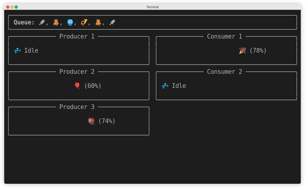
The script uses the Rich library, which you’ll need to install into your virtual environment first:
(venv) $ python -m pip install rich
This will let you add colors, emojis, and visual components to your terminal. Note that some terminals may not support this kind of rich text formatting. Remember that at any point, you can download the complete source code of the scripts mentioned in this tutorial by following the link below if you haven’t already:
Get Source Code: Click here to get access to the source code and sample data that you’ll use to explore queues in Python.
Before you start using queues, you’ll have to do a bit of scaffolding. Create a new file named thread_safe_queues.py and define the entry point to your script, which will parse arguments with the argparse module:
# thread_safe_queues.py

import argparse
from queue import LifoQueue, PriorityQueue, Queue

QUEUE_TYPES = {
    "fifo": Queue,
    "lifo": LifoQueue,
    "heap": PriorityQueue
}

def main(args):
    buffer = QUEUE_TYPES[args.queue]()

def parse_args():
    parser = argparse.ArgumentParser()
    parser.add_argument("-q", "--queue", choices=QUEUE_TYPES, default="fifo")
    parser.add_argument("-p", "--producers", type=int, default=3)
    parser.add_argument("-c", "--consumers", type=int, default=2)
    parser.add_argument("-ps", "--producer-speed", type=int, default=1)
    parser.add_argument("-cs", "--consumer-speed", type=int, default=1)
    return parser.parse_args()

if __name__ == "__main__":
    try:
        main(parse_args())
    except KeyboardInterrupt:
        pass
First, you import the necessary module and queue classes into the global namespace. The main() function is your entry point, which receives the parsed arguments supplied by parse_args(), which is defined below. The QUEUE_TYPES dictionary maps queue names to their respective classes, which you call to create a new queue instance based on the value of a command-line argument.
Next, you define the products that your producers will pick at random and pretend to be working on:
# thread_safe_queues.py

# ...

PRODUCTS = (
    ":balloon:",
    ":cookie:",
    ":crystal_ball:",
    ":diving_mask:",
    ":flashlight:",
    ":gem:",
    ":gift:",
    ":kite:",
    ":party_popper:",
    ":postal_horn:",
    ":ribbon:",
    ":rocket:",
    ":teddy_bear:",
    ":thread:",
    ":yo-yo:",
)

# ...
These are textual codes that Rich will eventually replace with the corresponding emoji glyphs. For example, :balloon: will render as 🎈. You can find all emoji codes available in Rich by running python -m rich.emoji in your terminal.
Your producer and consumer threads will share a wealth of attributes and behaviors, which you can encapsulate in a common base class:
# thread_safe_queues.py

import threading

# ...

class Worker(threading.Thread):
    def __init__(self, speed, buffer):
        super().__init__(daemon=True)
        self.speed = speed
        self.buffer = buffer
        self.product = None
        self.working = False
        self.progress = 0
The worker class extends the threading.Thread class and configures itself as a daemon thread so that its instances won’t prevent your program from exiting when the main thread finishes, for example, due to a keyboard interrupt signal. A worker object expects the speed rate to work with and a buffer queue to put finished products into or get them from.
In addition to that, you’ll be able to check the state of a worker thread and request that it simulate some work or idle time:
# thread_safe_queues.py

from random import randint
from time import sleep

# ...

class Worker(threading.Thread):
    # ...

    @property
    def state(self):
        if self.working:
            return f"{self.product} ({self.progress}%)"
        return ":zzz: Idle"

    def simulate_idle(self):
        self.product = None
        self.working = False
        self.progress = 0
        sleep(randint(1, 3))

    def simulate_work(self):
        self.working = True
        self.progress = 0
        delay = randint(1, 1 + 15 // self.speed)
        for _ in range(100):
            sleep(delay / 100)
            self.progress += 1
The .state property returns a string with either the product’s name and the progress of work or a generic message indicating that the worker is currently idle. The .simulate_idle() method resets the state of a worker thread and goes to sleep for a few randomly chosen seconds. Similarly, .simulate_work() picks a random delay in seconds adjusted to the worker’s speed and progresses through the work.
Studying the presentation layer based on the Rich library isn’t crucial to understanding this example, but feel free to expand the collapsible section below for more details:
The code below defines a view that renders the current state of your producers, consumers, and the queue ten times a second:
# thread_safe_queues.py

from itertools import zip_longest

from rich.align import Align
from rich.columns import Columns
from rich.console import Group
from rich.live import Live
from rich.panel import Panel

# ...

class View:
    def __init__(self, buffer, producers, consumers):
        self.buffer = buffer
        self.producers = producers
        self.consumers = consumers

    def animate(self):
        with Live(
            self.render(), screen=True, refresh_per_second=10
        ) as live:
            while True:
                live.update(self.render())

    def render(self):

        match self.buffer:
            case PriorityQueue():
                title = "Priority Queue"
                products = map(str, reversed(list(self.buffer.queue)))
            case LifoQueue():
                title = "Stack"
                products = list(self.buffer.queue)
            case Queue():
                title = "Queue"
                products = reversed(list(self.buffer.queue))
            case _:
                title = products = ""

        rows = [
            Panel(f"[bold]{title}:[/] {', '.join(products)}", width=82)
        ]
        pairs = zip_longest(self.producers, self.consumers)
        for i, (producer, consumer) in enumerate(pairs, 1):
            left_panel = self.panel(producer, f"Producer {i}")
            right_panel = self.panel(consumer, f"Consumer {i}")
            rows.append(Columns([left_panel, right_panel], width=40))
        return Group(*rows)

    def panel(self, worker, title):
        if worker is None:
            return ""
        padding = " " * int(29 / 100 * worker.progress)
        align = Align(
            padding + worker.state, align="left", vertical="middle"
        )
        return Panel(align, height=5, title=title)

# ...
Notice the use of structural pattern matching to set the title and products based on the queue type. You’ll create an instance of the view and call its .animate() method once the producers and consumers are in place.
Next up, you’ll define the producer and consumer classes, and connect the pieces together.
queue.Queue
The first synchronized queue that you’ll give a try is an unbounded FIFO queue or, simply put, a queue. You’ll need to pass it around to both your producers and consumers, so go ahead and define them now. The producer thread will extend a worker class and take an additional collection of products to choose from:
# thread_safe_queues.py

from random import choice, randint

# ...

class Producer(Worker):
    def __init__(self, speed, buffer, products):
        super().__init__(speed, buffer)
        self.products = products

    def run(self):
        while True:
            self.product = choice(self.products)
            self.simulate_work()
            self.buffer.put(self.product)
            self.simulate_idle()

# ...
The .run() method is where all the magic happens. A producer works in an infinite loop, choosing a random product and simulating some work before putting that product onto the queue, called a buffer. It then goes to sleep for a random period, and when it wakes up again, the process repeats.
A consumer is very similar, but even more straightforward than a producer:
# thread_safe_queues.py

# ...

class Consumer(Worker):
    def run(self):
        while True:
            self.product = self.buffer.get()
            self.simulate_work()
            self.buffer.task_done()
            self.simulate_idle()

# ...
It also works in an infinite loop, waiting for a product to appear in the queue. The .get() method is blocking by default, which will keep the consumer thread stopped and waiting until there’s at least one product in the queue. This way, a waiting consumer won’t be wasting any CPU cycles while the operating system allocates valuable resources to other threads doing useful work.
Note: To avoid a deadlock, you can optionally set a timeout on the .get() method by passing a timeout keyword argument with the number of seconds to wait before giving up.
Each time you get something from a synchronized queue, its internal counter increases to let other threads know the queue hasn’t been drained yet. Therefore, it’s important to mark a dequeued task as done when you’re finished processing it unless you don’t have any threads joining the queue. Doing so decreases the queue’s internal counter.
Now, go back to your main() function, create the producer and consumer threads, and start them:
# thread_safe_queues.py

# ...

def main(args):
    buffer = QUEUE_TYPES[args.queue]()
    producers = [
        Producer(args.producer_speed, buffer, PRODUCTS)
        for _ in range(args.producers)
    ]
    consumers = [
        Consumer(args.consumer_speed, buffer) for _ in range(args.consumers)
    ]

    for producer in producers:
        producer.start()

    for consumer in consumers:
        consumer.start()

    view = View(buffer, producers, consumers)
    view.animate()
The number of producers and consumers is determined by the command-line arguments passed into your function. They’ll begin working and using the queue for interthread communication as soon as you start them. The View instance at the bottom continually re-renders the screen to reflect the current state of your application:
Producers will always push their finished products through that queue to the consumers. Even though it may sometimes appear as if a consumer takes an element directly from a producer, it’s only because things are happening too fast to notice the enqueue and dequeue operations.
Note: It’s worth noting that whenever a producer puts something onto a synchronized queue, at most one consumer will dequeue that element and process it without other consumers ever knowing. If you wish to notify more than one consumer about a particular event in your program, then have a look at other thread coordination primitives in the threading module.
You can increase the number of producers, their speed, or both to see how these changes affect the overall capacity of your system. Because the queue is unbounded, it’ll never slow down the producers. However, if you specified the queue’s maxsize parameter, then it would start blocking them until there was enough space in the queue again.
Using a FIFO queue makes the producers put elements on the left end of the queue in the visualization above. At the same time, consumers compete with each other for the rightmost product in the queue. In the next section, you’ll see how this behavior changes when you call the script with the --queue lifo option.
queue.LifoQueue
From your workers’ perspective, there’s absolutely no need to make any changes to your code in order to modify how they communicate. Merely by injecting a different type of synchronized queue into them, you can modify the rules of the workers’ communication. Run your script with a LIFO queue now:
$ python thread_safe_queues.py --queue lifo
When you use a LIFO queue or a stack, each new product that has just been created will take precedence over the older ones in the queue:
In rare cases, when new products are created more quickly than your consumers can cope with them, older products might suffer from starvation because they get stuck at the bottom of the stack and never get consumed. On the other hand, that might not be a problem when you have a big enough consumer pool or when you don’t get as many incoming products. Starvation can also involve elements on a priority queue, which you’ll read about next.
queue.PriorityQueue
To use a synchronized priority queue or a heap, you’ll need to make a few adjustments in your code. First of all, you’re going to need a new kind of product that has an associated priority, so define two new data types:
# thread_safe_queues.py

from dataclasses import dataclass, field
from enum import IntEnum

# ...

@dataclass(order=True)
class Product:
    priority: int
    label: str = field(compare=False)

    def __str__(self):
        return self.label

class Priority(IntEnum):
    HIGH = 1
    MEDIUM = 2
    LOW = 3

PRIORITIZED_PRODUCTS = (
    Product(Priority.HIGH, ":1st_place_medal:"),
    Product(Priority.MEDIUM, ":2nd_place_medal:"),
    Product(Priority.LOW, ":3rd_place_medal:"),
)
To represent products, you use a data class with a customized string representation and ordering enabled, but you’re careful not to compare the products by their label. In this case, you expect the label to be a string, but generally, it could be any object that might not be comparable at all. You also define an enum class with known priority values and three products with descending priorities from highest to lowest.
Note: Contrary to your earlier priority queue implementation, Python’s thread-safe queue orders elements with the lowest numeric priority value first.
Additionally, when the user supplies the --queue heap option in the command line, then you must supply the right collection of products to your producer threads:
# thread_safe_queues.py

# ...

def main(args):
    buffer = QUEUE_TYPES[args.queue]()
    products = PRIORITIZED_PRODUCTS if args.queue == "heap" else PRODUCTS
    producers = [
        Producer(args.producer_speed, buffer, products)
        for _ in range(args.producers)
    ]
    # ...
You provide either plain or prioritized products depending on a command-line argument using a conditional expression.
The rest of your code can remain agnostic to this change as long as the producers and consumers know how to deal with a new product type. Because this is only a simulation, the worker threads don’t really do anything useful with the products, so you can run your script with the --queue heap flag and see the effect:
Remember that a heap data structure is a binary tree, which keeps a specific relationship between its elements. Therefore, even though the products in the priority queue don’t appear to be arranged quite correctly, they’re actually consumed in the right order. Also, because of the non-deterministic nature of multithreaded programming, Python queues don’t always report their most up-to-date size.
All right, you’ve witnessed the traditional way of coordinating worker threads using three types of synchronized queues. Python threads are well-suited to I/O-bound tasks, which spend most of their time waiting for data on the network, the file system, or a database. However, there’s recently been a single-threaded alternative to synchronized queues, taking advantage of Python’s asynchronous features. That’s what you’ll look at now.
Using Asynchronous Queues
If you’d like to use queues in an asynchronous context, then Python has you covered. The asyncio module provides asynchronous counterparts to queues from the threading module, which you can use in coroutine functions on a single thread. Because both queue families share a similar interface, switching from one to the other should be relatively painless.
In this section, you’ll write a rudimentary web crawler, which recursively follows links on a specified website up to a given depth level and counts the number of visits per link. To fetch data asynchronously, you’ll use the popular aiohttp library, and to parse HTML hyperlinks, you’ll rely on beautifulsoup4. Be sure to install both libraries into your virtual environment before proceeding:
(venv) $ python -m pip install aiohttp beautifulsoup4
Now you can make HTTP requests asynchronously and select HTML elements from a so-called tag soup received from the server.
Note: You can use Beautiful Soup and Python to build a web scraper, which collects valuable data while visiting web pages.
To lay the groundwork for your web crawler, you’ll make a few building blocks first. Create a new file named async_queues.py and define the following structure in it:
# async_queues.py

import argparse
import asyncio
from collections import Counter

import aiohttp

async def main(args):
    session = aiohttp.ClientSession()
    try:
        links = Counter()
        display(links)
    finally:
        await session.close()

def parse_args():
    parser = argparse.ArgumentParser()
    parser.add_argument("url")
    parser.add_argument("-d", "--max-depth", type=int, default=2)
    parser.add_argument("-w", "--num-workers", type=int, default=3)
    return parser.parse_args()

def display(links):
    for url, count in links.most_common():
        print(f"{count:>3} {url}")

if __name__ == "__main__":
    asyncio.run(main(parse_args()))
As with most asynchronous programs, you pass your main() coroutine to asyncio.run() so that it can execute it on the default event loop. The coroutine takes a few command-line arguments parsed with a helper function defined below, starts a new aiohttp.ClientSession, and defines a counter of the visited links. Later, the coroutine displays the list of links sorted by the number of visits in descending order.
To run your script, you’ll specify a root URL and optionally the maximum depth and the number of workers. Here’s an example:
$ python async_queues.py https://www.python.org/ --max-depth 2 \
                                                 --num-workers 3
There are still a few missing pieces like fetching content and parsing HTML links, so add them to your file:
# async_queues.py

from urllib.parse import urljoin
from bs4 import BeautifulSoup

# ...

async def fetch_html(session, url):
    async with session.get(url) as response:
        if response.ok and response.content_type == "text/html":
            return await response.text()

def parse_links(url, html):
    soup = BeautifulSoup(html, features="html.parser")
    for anchor in soup.select("a[href]"):
        href = anchor.get("href").lower()
        if not href.startswith("javascript:"):
            yield urljoin(url, href)
You’ll only return the received content as long as it’s HTML, which you can tell by looking at the Content-Type HTTP header. When extracting links from the HTML content, you’ll skip inline JavaScript in the href attribute, and optionally join a relative path with the current URL.
Next, you’re going to define a new data type representing a job that you’ll put in the queue, as well as an asynchronous worker performing the job:
# async_queues.py

import sys
from typing import NamedTuple

# ...

class Job(NamedTuple):
    url: str
    depth: int = 1

# ...

async def worker(worker_id, session, queue, links, max_depth):
    print(f"[{worker_id} starting]", file=sys.stderr)
    while True:
        url, depth = await queue.get()
        links[url] += 1
        try:
            if depth <= max_depth:
                print(f"[{worker_id} {depth=} {url=}]", file=sys.stderr)
                if html := await fetch_html(session, url):
                    for link_url in parse_links(url, html):
                        await queue.put(Job(link_url, depth + 1))
        except aiohttp.ClientError:
            print(f"[{worker_id} failed at {url=}]", file=sys.stderr)
        finally:
            queue.task_done()
A job consists of the URL address to visit and the current depth that a worker will use to stop crawling recursively. Thanks to specifying a job as a named tuple, you unpack its individual components on the highlighted line after dequeuing it. When you don’t specify the depth for a job, then it defaults to one.
The worker sits in an infinite loop, waiting for a job to arrive in the queue. After consuming a single job, the worker can put one or more new jobs with a bumped-up depth in the queue to be consumed by itself or other workers.
Because your worker is both a producer and a consumer, it’s crucial to unconditionally mark a job as done in a try … finally clause to avoid a deadlock. You should also handle errors in your worker because unhandled exceptions will make your worker stop accepting new jobs otherwise.
Note: You can use the print() function in asynchronous code—for example, to log diagnostic messages—because everything runs on a single thread. On the other hand, you’d have to replace it with the logging module in a multithreaded code because the print() function isn’t thread-safe.
Also, notice that you print the diagnostic messages to standard error (stderr), while the output of your program prints to standard output (stdout), which are two completely separate streams. This allows you to redirect one or both to a file, for instance.
Your worker increments the number of hits when visiting a URL. Additionally, if the current URL’s depth doesn’t exceed the maximum allowed depth, then the worker fetches the HTML content that the URL points to and iterates over its links. The walrus operator (:=) lets you await an HTTP response, check if the content was returned, and assign the result to the html variable in a single expression.
The last remaining step is to create an instance of the asynchronous queue and pass it to the workers.
asyncio.Queue
In this section, you’ll update your main() coroutine by creating the queue and the asynchronous tasks that run your workers. Each worker will receive a unique identifier to differentiate it in the log messages, an aiohttp session, the queue instance, the counter of visits to a particular link, and the maximum depth. Because you’re using a single thread, you don’t need to ensure mutually exclusive access to shared resources:
 1# async_queues.py
 2
 3# ...
 4
 5async def main(args):
 6    session = aiohttp.ClientSession()
 7    try:
 8        links = Counter()
 9        queue = asyncio.Queue()
10        tasks = [
11            asyncio.create_task(
12                worker(
13                    f"Worker-{i + 1}",
14                    session,
15                    queue,
16                    links,
17                    args.max_depth,
18                )
19            )
20            for i in range(args.num_workers)
21        ]
22
23        await queue.put(Job(args.url))
24        await queue.join()
25
26        for task in tasks:
27            task.cancel()
28
29        await asyncio.gather(*tasks, return_exceptions=True)
30
31        display(links)
32    finally:
33        await session.close()
34
35# ...
Here’s a line-by-line breakdown of the updated code:
- Line 9 instantiates an asynchronous FIFO queue.
- Lines 10 to 21 create a number of worker coroutines wrapped in asynchronous tasks that start running as soon as possible in the background on the event loop.
- Line 23 puts the first job in the queue, which kicks off the crawling.
- Line 24 causes the main coroutine to wait until the queue has been drained and there are no more jobs to perform.
- Lines 26 to 29 do a graceful cleanup when the background tasks are no longer needed.
Please, don’t run the web crawler against an actual website hosted online. It can cause an unwanted spike in the network traffic and get you in trouble. To test your crawler, you’re better off starting an HTTP server built into Python, which turns a local folder in your file system into a navigable website. For example, the following command will start a server in a local folder with a Python virtual environment:
$ cd venv/
$ python -m http.server
Serving HTTP on 0.0.0.0 port 8000 (http://0.0.0.0:8000/) ...
This isn’t an ideal analogy to a real-world website, though, because files and folders make up a tree-like hierarchy, whereas websites are often represented by dense multigraphs with backlinks. Anyway, when you run the web crawler against a chosen URL address in another terminal window, you’ll notice that the crawler follows the links in their natural order of appearance:
$ python async_queues.py http://localhost:8000 --max-depth=4
[Worker-1 starting]
[Worker-1 depth=1 url='http://localhost:8000']
[Worker-2 starting]
[Worker-3 starting]
[Worker-1 depth=2 url='http://localhost:8000/bin/']
[Worker-2 depth=2 url='http://localhost:8000/include/']
[Worker-3 depth=2 url='http://localhost:8000/lib/']
[Worker-2 depth=2 url='http://localhost:8000/lib64/']
[Worker-1 depth=2 url='http://localhost:8000/pyvenv.cfg']
[Worker-3 depth=3 url='http://localhost:8000/bin/activate']
[Worker-2 depth=3 url='http://localhost:8000/bin/activate.csh']
[Worker-1 depth=3 url='http://localhost:8000/bin/activate.fish']
[Worker-3 depth=3 url='http://localhost:8000/bin/activate.ps1']
[Worker-2 depth=3 url='http://localhost:8000/bin/pip']
[Worker-3 depth=3 url='http://localhost:8000/bin/pip3']
[Worker-1 depth=3 url='http://localhost:8000/bin/pip3.10']
[Worker-2 depth=3 url='http://localhost:8000/bin/python']
[Worker-3 depth=3 url='http://localhost:8000/bin/python3']
[Worker-1 depth=3 url='http://localhost:8000/bin/python3.10']
[Worker-2 depth=3 url='http://localhost:8000/lib/python3.10/']
[Worker-3 depth=3 url='http://localhost:8000/lib64/python3.10/']
[Worker-2 depth=4 url='http://localhost:8000/lib/python3.10/site-packages/']
[Worker-3 depth=4 url='http://localhost:8000/lib64/python3.10/site-packages/']
⋮
It visits the only URL on the first level with depth equal to one. Then, after visiting all links on the second level, the crawler proceeds to the third level and so on until reaching the maximum depth level requested. Once all links on a given level are explored, the crawler never goes back to an earlier level. That’s a direct consequence of using a FIFO queue, which is different from using a stack or a LIFO queue.
asyncio.LifoQueue
As with the synchronized queues, their asynchronous companions let you change the behavior of your workers without modifying their code. Go back to your async_queues module and replace the existing FIFO queue with a LIFO one:
# async_queues.py

# ...

async def main(args):
    session = aiohttp.ClientSession()
    try:
        links = Counter()
        queue = asyncio.LifoQueue()
        tasks = [
            asyncio.create_task(
                worker(
                    f"Worker-{i + 1}",
                    session,
                    queue,
                    links,
                    args.max_depth,
                )
            )
            for i in range(args.num_workers)
        ]

        await queue.put(Job(args.url))
        await queue.join()

        for task in tasks:
            task.cancel()

        await asyncio.gather(*tasks, return_exceptions=True)

        display(links)
    finally:
        await session.close()

# ...
Without stopping your HTTP server, run the web crawler using the same options again:
$ python async_queues.py http://localhost:8000 --max-depth=4
[Worker-1 starting]
[Worker-1 depth=1 url='http://localhost:8000']
[Worker-2 starting]
[Worker-3 starting]
[Worker-1 depth=2 url='http://localhost:8000/pyvenv.cfg']
[Worker-2 depth=2 url='http://localhost:8000/lib64/']
[Worker-3 depth=2 url='http://localhost:8000/lib/']
[Worker-1 depth=2 url='http://localhost:8000/include/']
[Worker-2 depth=3 url='http://localhost:8000/lib64/python3.10/']
[Worker-3 depth=3 url='http://localhost:8000/lib/python3.10/']
[Worker-1 depth=2 url='http://localhost:8000/bin/']
[Worker-2 depth=4 url='http://localhost:8000/lib64/python3.10/site-packages/']
[Worker-1 depth=3 url='http://localhost:8000/bin/python3.10']
[Worker-2 depth=3 url='http://localhost:8000/bin/python3']
[Worker-3 depth=4 url='http://localhost:8000/lib/python3.10/site-packages/']
[Worker-1 depth=3 url='http://localhost:8000/bin/python']
[Worker-2 depth=3 url='http://localhost:8000/bin/pip3.10']
[Worker-1 depth=3 url='http://localhost:8000/bin/pip3']
[Worker-3 depth=3 url='http://localhost:8000/bin/pip']
[Worker-2 depth=3 url='http://localhost:8000/bin/activate.ps1']
[Worker-1 depth=3 url='http://localhost:8000/bin/activate.fish']
[Worker-3 depth=3 url='http://localhost:8000/bin/activate.csh']
[Worker-2 depth=3 url='http://localhost:8000/bin/activate']
⋮
Assuming the content hasn’t changed since the last run, the crawler visits identical links but in a different order. The highlighted lines indicate visiting a link on a previously explored depth level.
Note: If you kept track of the already visited links and skipped them on the subsequent encounters, then it could lead to different outputs depending on the queue type used. That’s because many alternative paths might originate on different depth levels but lead up to the same destination.
Next up, you’ll see an asynchronous priority queue in action.
asyncio.PriorityQueue
To use your jobs in a priority queue, you must specify how to compare them when deciding on their priorities. For example, you may want to visit shorter URLs first. Go ahead and add the .__lt__() special method to your Job class, to which the less than (<) operator delegates when comparing two job instances:
# async_queues.py

# ...

class Job(NamedTuple):
    url: str
    depth: int = 1

    def __lt__(self, other):
        if isinstance(other, Job):
            return len(self.url) < len(other.url)
If you compare a job to a completely different data type, then you can’t say which one is smaller, so you implicitly return None. On the other hand, when comparing two instances of the Job class, you resolve their priorities by examining the lengths of their corresponding .url fields:
>>> from async_queues import Job
>>> job1 = Job("http://localhost/")
>>> job2 = Job("https://localhost:8080/")
>>> job1 < job2
True
The shorter the URL, the higher the priority because smaller values take precedence in a min-heap.
The last change to make in your script is using the asynchronous priority queue instead of the other two:
# async_queues.py

# ...

async def main(args):
    session = aiohttp.ClientSession()
    try:
        links = Counter()
        queue = asyncio.PriorityQueue()
        tasks = [
            asyncio.create_task(
                worker(
                    f"Worker-{i + 1}",
                    session,
                    queue,
                    links,
                    args.max_depth,
                )
            )
            for i in range(args.num_workers)
        ]

        await queue.put(Job(args.url))
        await queue.join()

        for task in tasks:
            task.cancel()

        await asyncio.gather(*tasks, return_exceptions=True)

        display(links)
    finally:
        await session.close()

# ...
Try running your web crawler with an even bigger maximum depth value—say, five:
$ python async_queues.py http://localhost:8000 --max-depth 5
[Worker-1 starting]
[Worker-1 depth=1 url='http://localhost:8000']
[Worker-2 starting]
[Worker-3 starting]
[Worker-1 depth=2 url='http://localhost:8000/bin/']
[Worker-2 depth=2 url='http://localhost:8000/lib/']
[Worker-3 depth=2 url='http://localhost:8000/lib64/']
[Worker-3 depth=2 url='http://localhost:8000/include/']
[Worker-2 depth=2 url='http://localhost:8000/pyvenv.cfg']
[Worker-1 depth=3 url='http://localhost:8000/bin/pip']
[Worker-3 depth=3 url='http://localhost:8000/bin/pip3']
[Worker-2 depth=3 url='http://localhost:8000/bin/python']
[Worker-1 depth=3 url='http://localhost:8000/bin/python3']
[Worker-3 depth=3 url='http://localhost:8000/bin/pip3.10']
[Worker-2 depth=3 url='http://localhost:8000/bin/activate']
[Worker-1 depth=3 url='http://localhost:8000/bin/python3.10']
[Worker-3 depth=3 url='http://localhost:8000/lib/python3.10/']
[Worker-2 depth=3 url='http://localhost:8000/bin/activate.ps1']
[Worker-3 depth=3 url='http://localhost:8000/bin/activate.csh']
[Worker-1 depth=3 url='http://localhost:8000/lib64/python3.10/']
[Worker-2 depth=3 url='http://localhost:8000/bin/activate.fish']
[Worker-3 depth=4 url='http://localhost:8000/lib/python3.10/site-packages/']
[Worker-1 depth=4 url='http://localhost:8000/lib64/python3.10/site-packages/']
⋮
You’ll immediately notice that links are generally explored in the order determined by the URL lengths. Naturally, the exact order will vary slightly with each run because of the non-deterministic nature of the time it takes for the server to reply.
Asynchronous queues are a fairly new addition to the Python standard library. They deliberately mimic an interface of the corresponding thread-safe queues, which should make any seasoned Pythonista feel at home. You can use asynchronous queues to exchange data between coroutines.
In the next section, you’ll familiarize yourself with the last family of queues available in the Python standard library, which lets you communicate across two or more OS-level processes.
Using multiprocessing.Queue for Interprocess Communication (IPC)
So far, you’ve looked into queues that can only help in scenarios with strictly I/O-bound tasks, whose progress doesn’t depend on the available computational power. On the other hand, the traditional approach to running CPU-bound tasks on multiple CPU cores in parallel with Python takes advantage of cloning the interpreter process. Your operating system provides the interprocess communication (IPC) layer for sharing data across these processes.
For example, you can start a new Python process with multiprocessing or use a pool of such processes from the concurrent.futures module. Both modules are carefully designed to make the switch from threads to processes as smooth as possible, which makes parallelizing your existing code rather straightforward. In some cases, it’s just a matter of replacing an import statement because the rest of the code follows a standard interface.
You’ll only find the FIFO queue in the multiprocessing module, which comes in three variants:
multiprocessing.Queuemultiprocessing.SimpleQueuemultiprocessing.JoinableQueue
They’re all modeled after the thread-based queue.Queue but differ in the level of completeness. The JoinableQueue extends the multiprocessing.Queue class by adding .task_done() and .join() methods, allowing you to wait until all enqueued tasks have been processed. If you don’t need this feature, then use multiprocessing.Queue instead. SimpleQueue is a separate, significantly streamlined class that only has .get(), .put(), and .empty() methods.
Note: Sharing a resource, such as a queue, between operating system processes is much more expensive and limited than sharing between threads. Unlike threads, processes don’t share a common memory region, so data must be marshaled and unmarshaled at both ends every time you pass a message from one process to another.
Moreover, Python uses the pickle module for data serialization, which doesn’t handle every data type and is relatively slow and insecure. As a result of that, you should only consider multiple processes when the performance improvements by running your code in parallel can offset the additional data serialization and bootstrapping overhead.
To see a hands-on example of multiprocessing.Queue, you’ll simulate a computationally intensive task by trying to reverse an MD5 hash value of a short text using the brute-force approach. While there are better ways to solve this problem, both algorithmically and programmatically, running more than one process in parallel will let you noticeably reduce the processing time.
Reversing an MD5 Hash on a Single Thread
Before parallelizing your computation, you’ll focus on implementing a single-threaded version of the algorithm and measuring the execution time against some test input. Create a new Python module named multiprocess_queue and place the following code in it:
 1# multiprocess_queue.py
 2
 3import time
 4from hashlib import md5
 5from itertools import product
 6from string import ascii_lowercase
 7
 8def reverse_md5(hash_value, alphabet=ascii_lowercase, max_length=6):
 9    for length in range(1, max_length + 1):
10        for combination in product(alphabet, repeat=length):
11            text_bytes = "".join(combination).encode("utf-8")
12            hashed = md5(text_bytes).hexdigest()
13            if hashed == hash_value:
14                return text_bytes.decode("utf-8")
15
16def main():
17    t1 = time.perf_counter()
18    text = reverse_md5("a9d1cbf71942327e98b40cf5ef38a960")
19    print(f"{text} (found in {time.perf_counter() - t1:.1f}s)")
20
21if __name__ == "__main__":
22    main()
Lines 8 to 14 define a function that’ll try to reverse an MD5 hash value provided as the first argument. By default, the function only considers text comprising up to six lowercase ASCII letters. You can change the alphabet and the maximum length of the text to guess by providing two other optional arguments.
For every possible combination of letters in the alphabet with the given length, reverse_md5() calculates a hash value and compares it against the input. If there’s a match, then it stops and returns the guessed text.
Note: Nowadays, MD5 is considered cryptographically unsafe because you can calculate such digests rapidly. Yet, six characters pulled from twenty-six ASCII letters gives a total of 308,915,776 distinct combinations, which is plenty for a Python program.
Lines 16 to 19 call the function with a sample MD5 hash value passed as an argument and measure its execution time using a Python timer. On a veteran desktop computer, it can take a few seconds to find a combination that hashes to the specified input:
$ python multiprocess_queue.py
queue (found in 6.9s)
As you can see, the word queue is the answer because it has an MD5 digest that matches your hard-coded hash value on line 18. Seven seconds isn’t terrible, but you can probably do better by taking advantage of your idle CPU cores, which are eager to do some work for you. To leverage their potential, you must chunk the data and distribute it to your worker processes.
Distributing Workload Evenly in Chunks
You want to narrow down the search space in each worker by dividing the whole set of letter combinations into a few smaller disjoint subsets. To ensure that workers don’t waste time doing work that’s already been done by another worker, the sets can’t have any overlap. While you don’t know the size of an individual chunk, you can provide a number of chunks equal to the number of CPU cores.
To calculate indices of the subsequent chunks, use the helper function below:
# multiprocess_queue.py

# ...

def chunk_indices(length, num_chunks):
    start = 0
    while num_chunks > 0:
        num_chunks = min(num_chunks, length)
        chunk_size = round(length / num_chunks)
        yield start, (start := start + chunk_size)
        length -= chunk_size
        num_chunks -= 1
It yields tuples consisting of the first index of the current chunk and its last index increased by one, making the tuple convenient to use as input to the built-in range() function. Because of rounding of the subsequent chunk lengths, those with varying lengths end up nicely interleaved:
>>> from multiprocess_queue import chunk_indices
>>> for start, stop in chunk_indices(20, 6):
...     print(len(r := range(start, stop)), r)
...
3 range(0, 3)
3 range(3, 6)
4 range(6, 10)
3 range(10, 13)
4 range(13, 17)
3 range(17, 20)
For example, a total length of twenty divided into six chunks yields indices that alternate between three and four elements.
To minimize the cost of data serialization between your processes, each worker will produce its own chunk of letter combinations based on the range of indices specified in a dequeued job object. You’ll want to find a letter combination or an n-tuple of m-set for a particular index. To make your life easier, you can encapsulate the formula for the combination in a new class:
# multiprocess_queue.py

# ...

class Combinations:
    def __init__(self, alphabet, length):
        self.alphabet = alphabet
        self.length = length

    def __len__(self):
        return len(self.alphabet) ** self.length

    def __getitem__(self, index):
        if index >= len(self):
            raise IndexError
        return "".join(
            self.alphabet[
                (index // len(self.alphabet) ** i) % len(self.alphabet)
            ]
            for i in reversed(range(self.length))
        )
This custom data type represents a collection of alphabet letter combinations with a given length. Thanks to the two special methods and raising the IndexError exception when all combinations are exhausted, you can iterate over instances of the Combinations class using a loop.
The formula above determines the character at a given position in a combination specified by an index, much like an odometer works in a car or a positional system in math. The letters in the rightmost position change most frequently, while letters change less often the further left they are.
You can now update your MD5-reversing function to use the new class and remove the itertools.product import statement:
# multiprocess_queue.py

# ...

def reverse_md5(hash_value, alphabet=ascii_lowercase, max_length=6):
    for length in range(1, max_length + 1):
        for combination in Combinations(alphabet, length):
            text_bytes = "".join(combination).encode("utf-8")
            hashed = md5(text_bytes).hexdigest()
            if hashed == hash_value:
                return text_bytes.decode("utf-8")

# ...
Unfortunately, replacing a built-in function implemented in C with a pure-Python one and doing some calculations in Python make the code an order of magnitude slower:
$ python multiprocess_queue.py
queue (found in 38.8s)
There are a few optimizations that you could make to gain a few seconds. For example, you might implement .__iter__() in your Combinations class to avoid making the if statement or raising an exception. You could also store the alphabet’s length as an instance attribute. However, these optimizations aren’t important for the sake of the example.
Next up, you’ll create the worker process, job data type, and two separate queues to communicate between the main process and its children.
Communicating in Full-Duplex Mode
Each worker process will have a reference to the input queue with jobs to consume and a reference to the output queue for the prospective solution. These references enable simultaneous two-way communication between workers and the main process, known as full-duplex communication. To define a worker process, you extend the Process class, which provides the familiar .run() method, just like a thread:
# multiprocess_queue.py

import multiprocessing

# ...

class Worker(multiprocessing.Process):
    def __init__(self, queue_in, queue_out, hash_value):
        super().__init__(daemon=True)
        self.queue_in = queue_in
        self.queue_out = queue_out
        self.hash_value = hash_value

    def run(self):
        while True:
            job = self.queue_in.get()
            if plaintext := job(self.hash_value):
                self.queue_out.put(plaintext)
                break

# ...
Later, the main process will periodically check whether one of the workers has placed a reversed MD5 text on the output queue and terminate the program early in such a case. The workers are daemons, so they won’t hold up the main process. Also notice that workers store the input hash value to reverse.
Add a Job class that Python will serialize and place on the input queue for worker processes to consume:
# multiprocess_queue.py

from dataclasses import dataclass

# ...

@dataclass(frozen=True)
class Job:
    combinations: Combinations
    start_index: int
    stop_index: int

    def __call__(self, hash_value):
        for index in range(self.start_index, self.stop_index):
            text_bytes = self.combinations[index].encode("utf-8")
            hashed = md5(text_bytes).hexdigest()
            if hashed == hash_value:
                return text_bytes.decode("utf-8")
By implementing the special method .__call__() in a job, you make objects of your class callable. Thanks to that, the workers can call these jobs just like regular functions when they receive them. The method’s body is similar to but slightly different from reverse_md5(), which you can remove now because you won’t need it anymore.
Finally, create both queues and populate the input queue with jobs before starting your worker processes:
# multiprocess_queue.py

import argparse

# ...

def main(args):
    queue_in = multiprocessing.Queue()
    queue_out = multiprocessing.Queue()

    workers = [
        Worker(queue_in, queue_out, args.hash_value)
        for _ in range(args.num_workers)
    ]

    for worker in workers:
        worker.start()

    for text_length in range(1, args.max_length + 1):
        combinations = Combinations(ascii_lowercase, text_length)
        for indices in chunk_indices(len(combinations), len(workers)):
            queue_in.put(Job(combinations, *indices))

def parse_args():
    parser = argparse.ArgumentParser()
    parser.add_argument("hash_value")
    parser.add_argument("-m", "--max-length", type=int, default=6)
    parser.add_argument(
        "-w",
        "--num-workers",
        type=int,
        default=multiprocessing.cpu_count(),
    )
    return parser.parse_args()

# ...

if __name__ == "__main__":
    main(parse_args())
As in the earlier examples, you parse the command-line arguments using the argparse module. The only mandatory argument for your script is the hash value to reverse, such as:
(venv) $ python multiprocess_queue.py a9d1cbf71942327e98b40cf5ef38a960
You can optionally specify the number of worker processes using the --num-workers command-line parameter, which defaults to the number of your CPU cores. There’s usually no benefit in cranking up the number of workers above the number of physical or logical processing units in hardware because of the additional cost of context switching, which starts to add up.
On the other hand, context switching becomes almost negligible in I/O-bound tasks, where you might end up having thousands of worker threads or coroutines. Processes are a different story because they’re much more expensive to create. Even if you front-load this cost using a process pool, there are certain limits.
At this point, your workers engage in two-way communication with the main process through the input and output queues. However, the program exits abruptly right after starting because the main process ends without waiting for its daemon children to finish processing their jobs. Now is the time to periodically poll the output queue for a potential solution and break out of the loop when you find one:
 1# multiprocess_queue.py
 2
 3import queue
 4import time
 5
 6# ...
 7
 8def main(args):
 9    t1 = time.perf_counter()
10
11    queue_in = multiprocessing.Queue()
12    queue_out = multiprocessing.Queue()
13
14    workers = [
15        Worker(queue_in, queue_out, args.hash_value)
16        for _ in range(args.num_workers)
17    ]
18
19    for worker in workers:
20        worker.start()
21
22    for text_length in range(1, args.max_length + 1):
23        combinations = Combinations(ascii_lowercase, text_length)
24        for indices in chunk_indices(len(combinations), len(workers)):
25            queue_in.put(Job(combinations, *indices))
26
27    while any(worker.is_alive() for worker in workers):
28        try:
29            solution = queue_out.get(timeout=0.1)
30            if solution:
31                t2 = time.perf_counter()
32                print(f"{solution} (found in {t2 - t1:.1f}s)")
33                break
34        except queue.Empty:
35            pass
36    else:
37        print("Unable to find a solution")
38
39# ...
You set the optional timeout parameter on the queue’s .get() method to avoid blocking and allow the while-loop to run its condition. When a solution is found, you dequeue it from the output queue, print the matched text on the standard output along with the estimated execution time, and break out of the loop. Note that multiprocessing.Queue raises exceptions defined in the queue module, which you might need to import.
However, when there’s no matching solution, the loop will never stop because your workers are still alive, waiting for more jobs to process even after having consumed all of them. They’re stuck on the queue_in.get() call, which is blocking. You’ll fix that in the upcoming section.
Killing a Worker With the Poison Pill
Because the number of jobs to consume is known up front, you can tell the workers to shut down gracefully after draining the queue. A typical pattern to request a thread or process stop working is by putting a special sentinel value at the end of the queue. Whenever a worker finds that sentinel, it’ll do the necessary cleanup and escape the infinite loop. Such a sentinel is known as the poison pill because it kills the worker.
Choosing the value for a sentinel can be tricky, especially with the multiprocessing module because of how it handles the global namespace. Check out the programming guidelines in the official documentation for more details. It’s probably safest to stick to a predefined value such as None, which has a known identity everywhere:
# multiprocess_queue.py

POISON_PILL = None

# ...
If you used a custom object() instance defined as a global variable, then each of your worker processes would have its own copy of that object with a unique identity. A sentinel object enqueued by one worker would be deserialized into an entirely new instance in another worker, having a different identity than its global variable. Therefore, you wouldn’t be able to detect a poison pill in the queue.
Another nuance to watch out for is taking care to put the poison pill back in the source queue after consuming it:
# multiprocess_queue.py

# ...

class Worker(multiprocessing.Process):
    def __init__(self, queue_in, queue_out, hash_value):
        super().__init__(daemon=True)
        self.queue_in = queue_in
        self.queue_out = queue_out
        self.hash_value = hash_value

    def run(self):
        while True:
            job = self.queue_in.get()
            if job is POISON_PILL:
                self.queue_in.put(POISON_PILL)
                break
            if plaintext := job(self.hash_value):
                self.queue_out.put(plaintext)
                break

# ...
This will give other workers a chance to consume the poison pill. Alternatively, if you know the exact number of your workers, then you can enqueue that many poison pills, one for each of them. After consuming and returning the sentinel to the queue, a worker breaks out of the infinite loop, ending its life.
Finally, don’t forget to add the poison pill as the last element in the input queue:
# multiprocess_queue.py

# ...

def main(args):
    t1 = time.perf_counter()

    queue_in = multiprocessing.Queue()
    queue_out = multiprocessing.Queue()

    workers = [
        Worker(queue_in, queue_out, args.hash_value)
        for _ in range(args.num_workers)
    ]

    for worker in workers:
        worker.start()

    for text_length in range(1, args.max_length + 1):
        combinations = Combinations(ascii_lowercase, text_length)
        for indices in chunk_indices(len(combinations), len(workers)):
            queue_in.put(Job(combinations, *indices))

    queue_in.put(POISON_PILL)

    while any(worker.is_alive() for worker in workers):
        try:
            solution = queue_out.get(timeout=0.1)
            t2 = time.perf_counter()
            if solution:
                print(f"{solution} (found in {t2 - t1:.1f}s)")
                break
        except queue.Empty:
            pass
    else:
        print("Unable to find a solution")

# ...
Now, your script is complete and can handle finding a matching text as well as facing situations when the MD5 hash value can’t be reversed. In the next section, you’ll run a few benchmarks to see whether this whole exercise was worth the effort.
Analyzing the Performance of Parallel Execution
When you compare the speed of execution of your original single-threaded version and the multiprocessing one, then you might get disappointed. While you took care to minimize the data serialization cost, rewriting bits of code to pure Python was the real bottleneck.
What’s even more surprising is that the speed seems to vary with changing input hash values as well as the number of worker processes:
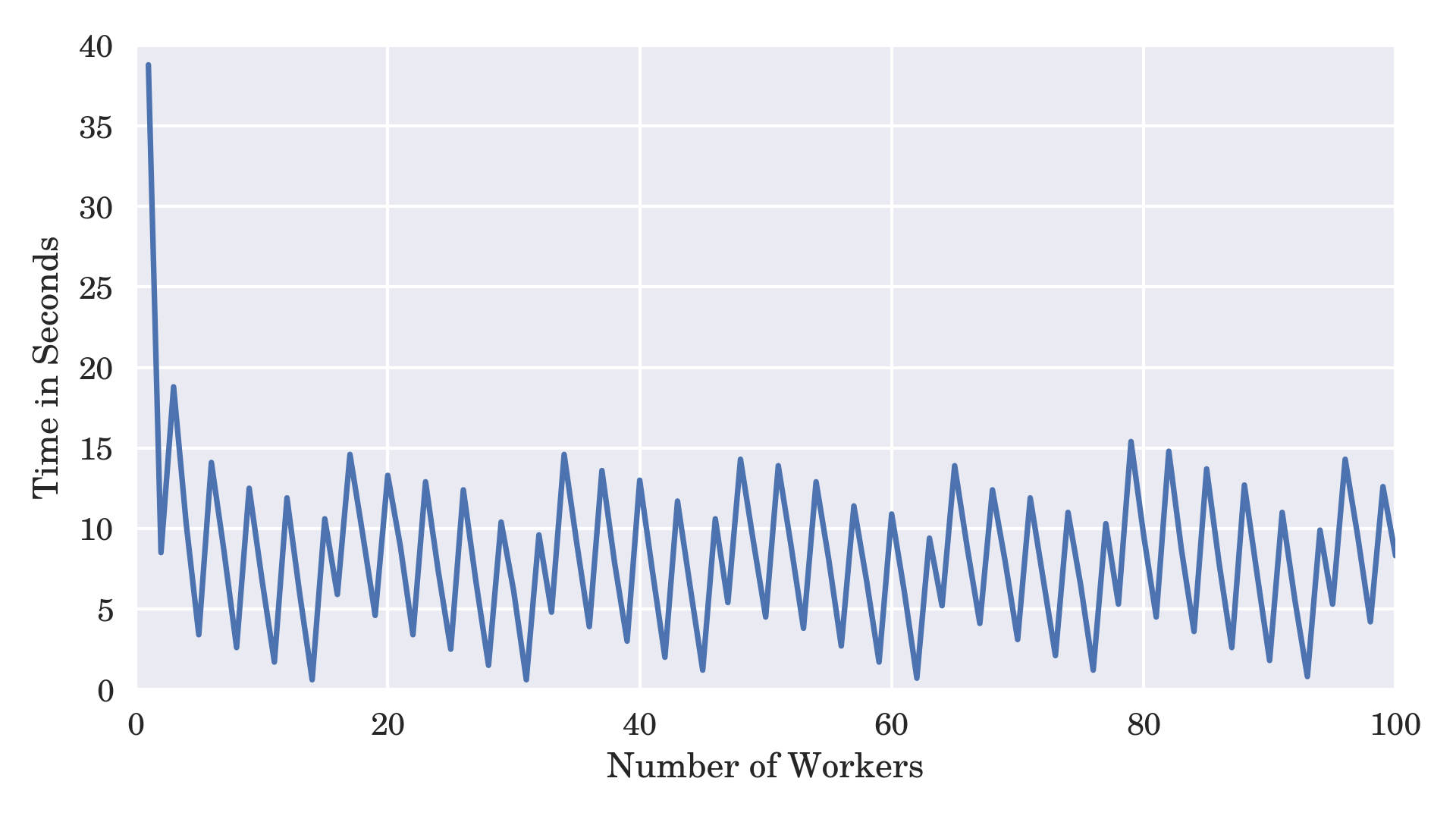
You would think that increasing the number of workers would decrease the overall computation time, and it does to a certain extent. There’s a huge drop from the single worker to multiple workers. However, the execution times periodically jump back and forth somewhat as you add more workers. There are a few factors at play here.
Primarily, the lucky worker that gets assigned a chunk containing your solution will run longer if the matching combination is located near the end of that chunk. Depending on the division points in your search space, which stem from the number of workers, you’ll get a different distance to the solution in a chunk. Secondly, the more workers you create, the bigger the impact context switching starts to have, even if the distance remains the same.
On the other hand, if all of your workers always had the same amount of work to do, then you’d observe a roughly linear trend without the sudden jumps. As you can see, parallelizing the execution of Python code isn’t always a straightforward process. That said, with a little bit of patience and persistence, you can most definitely optimize those few bottlenecks. For example, you could:
- Figure out a more clever formula
- Trade memory for speed by caching and pre-calculating intermediate results
- Inline function calls and other expensive constructs
- Find a third-party C library with Python bindings
- Write a Python C extension module or use ctypes or Cython
- Bring just-in-time (JIT) compilation tools for Python
- Switch to an alternative Python interpreter like PyPy
At this point, you’ve covered all queue types available in the Python standard library, including synchronized thread-safe queues, asynchronous queues, and a FIFO queue for process-based parallelism. In the next section, you’ll take a brief look at a few third-party libraries that’ll let you integrate with standalone message queue brokers.
Integrating Python With Distributed Message Queues
In distributed systems with a lot of moving parts, it’s often desirable to decouple your application components using an intermediate message broker, which takes the burden of resilient message delivery between the producer and consumer services. It typically requires its own infrastructure, which is both an advantage and a disadvantage.
On the one hand, it’s yet another abstraction layer that adds complexity and needs maintenance, but when configured correctly, it can provide these benefits:
- Loose Coupling: You can modify or replace one component with another without affecting the rest of your system.
- Flexibility: You can alter your system’s business rules by changing the broker configuration and message delivery rules without writing code.
- Scalability: You can dynamically add more components of a given kind to handle the increased workload in a specific functional area.
- Reliability: Consumers may need to acknowledge a message before the broker removes it from a queue to ensure safe delivery. Running the broker in the cluster may provide additional fault tolerance.
- Persistence: The broker may keep some messages in the queue while the consumers are offline due to a failure.
- Performance: Using a dedicated infrastructure for the message broker offloads your application services.
There are many different types of message brokers and scenarios in which you can use them. In this section, you’ll get a taste of a few of them.
RabbitMQ: pika
RabbitMQ is probably one of the most popular open source message brokers, which lets you route messages from producers to consumers in several ways. You can conveniently start a new RabbitMQ broker without installing it on your computer by running a temporary Docker container:
$ docker run -it --rm --name rabbitmq -p 5672:5672 rabbitmq
Once it’s started, you can connect to it on your localhost and the default port 5672. The official documentation recommends using the Pika library for connecting to a RabbitMQ instance in Python. This is what a rudimentary producer can look like:
# producer.py

import pika

QUEUE_NAME = "mailbox"

with pika.BlockingConnection() as connection:
    channel = connection.channel()
    channel.queue_declare(queue=QUEUE_NAME)
    while True:
        message = input("Message: ")
        channel.basic_publish(
            exchange="",
            routing_key=QUEUE_NAME,
            body=message.encode("utf-8")
        )
You open a connection using the default parameters, which assume that RabbitMQ is already running on your local machine. Then, you create a new channel, which is a lightweight abstraction on top of a TCP connection. You can have multiple independent channels for separate transmissions. Before entering the loop, you make sure that a queue named mailbox exists in the broker. Finally, you keep publishing messages read from the user.
The consumer is only slightly longer, as it requires defining a callback function to process the messages:
# consumer.py

import pika

QUEUE_NAME = "mailbox"

def callback(channel, method, properties, body):
    message = body.decode("utf-8")
    print(f"Got message: {message}")

with pika.BlockingConnection() as connection:
    channel = connection.channel()
    channel.queue_declare(queue=QUEUE_NAME)
    channel.basic_consume(
        queue=QUEUE_NAME,
        auto_ack=True,
        on_message_callback=callback
    )
    channel.start_consuming()
Most of the boilerplate code looks similar to your producer. However, you don’t need to write an explicit loop because the consumer will listen for messages indefinitely.
Go ahead and start a few producers and consumers in separate terminal tabs. Notice what happens when the first consumer connects to RabbitMQ after the queue already has some unconsumed messages or if you have more than one consumer connected to the broker.
Redis: redis
Redis is short for Remote Dictionary Server, but it’s really many things in disguise. It’s an in-memory key-value data store that usually works as an ultra-fast cache between a traditional SQL database and a server. At the same time, it can serve as a persistent NoSQL database and also a message broker in the publish-subscribe model. You can start a local Redis server with Docker:
$ docker run -it --rm --name redis -p 6379:6379 redis
When you do, you’ll be able to connect to a running container using the Redis command-line interface:
$ docker exec -it redis redis-cli
127.0.0.1:6379>
Take a look at the list of commands in the official documentation and try them out while you’re connected to the Redis server. Alternatively, you can jump right into Python. The first library listed on the official Redis page is redis, but it’s worth noting that you can choose from many alternatives, including asynchronous ones.
Writing a bare-bones publisher doesn’t take more than a couple of lines of Python code:
# publisher.py

import redis

with redis.Redis() as client:
    while True:
        message = input("Message: ")
        client.publish("chatroom", message)
You connect to a local Redis server instance and immediately start publishing messages on the chatroom channel. You don’t have to create the channels, because Redis will do it for you. Subscribing to a channel requires one extra step, creating the PubSub object to call the .subscribe() method on:
# subscriber.py

import redis

with redis.Redis() as client:
    pubsub = client.pubsub()
    pubsub.subscribe("chatroom")
    for message in pubsub.listen():
        if message["type"] == "message":
            body = message["data"].decode("utf-8")
            print(f"Got message: {body}")
Messages received by a subscriber are Python dictionaries with some metadata, which lets you decide how to deal with them. If you have multiple active subscribers listening on a channel, then all of them will receive the same message. On the other hand, messages aren’t persisted by default.
Check out How to Use Redis With Python to learn more.
Apache Kafka: kafka-python3
Kafka is by far the most advanced and complicated of the three message brokers you’ll meet in this tutorial. It’s a distributed streaming platform used in real-time event-driven applications. Its main selling point is the ability to handle large volumes of data with almost no performance lag.
To run Kafka, you’ll need to set up a distributed cluster. You may use Docker Compose to start a multi-container Docker application in one go. For example, you can grab Apache Kafka packaged by Bitnami:
# docker-compose.yml

version: "3"
services:
  zookeeper:
    image: 'bitnami/zookeeper:latest'
    ports:
      - '2181:2181'
    environment:
      - ALLOW_ANONYMOUS_LOGIN=yes
  kafka:
    image: 'bitnami/kafka:latest'
    ports:
      - '9092:9092'
    environment:
      - KAFKA_BROKER_ID=1
      - KAFKA_CFG_LISTENERS=PLAINTEXT://:9092
      - KAFKA_CFG_ADVERTISED_LISTENERS=PLAINTEXT://127.0.0.1:9092
      - KAFKA_CFG_ZOOKEEPER_CONNECT=zookeeper:2181
      - ALLOW_PLAINTEXT_LISTENER=yes
    depends_on:
      - zookeeper
When you save this configuration in a file named docker-compose.yml, then you can start the two services by running the command below:
$ docker-compose up
Sometimes, you may run into issues when the Kafka version doesn’t match the version of your client library. The Python library that seems to support a fairly recent Kafka is kafka-python3, modeled on the Java client.
Your producer can send messages on a given topic like so:
# producer.py

from kafka3 import KafkaProducer

producer = KafkaProducer(bootstrap_servers="localhost:9092")
while True:
    message = input("Message: ")
    producer.send(
        topic="datascience",
        value=message.encode("utf-8"),
    )
The .send() method is asynchronous because it returns a future object that you can await by calling its blocking .get() method. On the consumer’s side, you’ll be able to read the sent messages by iterating over the consumer:
# consumer.py

from kafka3 import KafkaConsumer

consumer = KafkaConsumer("datascience")
for record in consumer:
    message = record.value.decode("utf-8")
    print(f"Got message: {message}")
The consumer’s constructor takes one or more topics that it might be interested in.
Naturally, you barely scratched the surface with what’s possible with these powerful message brokers. Your goal in this section was to get a quick overview and a starting point in case you’d like to explore them on your own.
Conclusion
Now you have a solid understanding of the theory of queues in computer science and know their practical uses, ranging from finding the shortest path in a graph to synchronizing concurrent workers and decoupling distributed systems. You’re able to recognize problems that queues can elegantly solve.
You can implement FIFO, LIFO, and priority queues from scratch using different data structures in Python, understanding their trade-offs. At the same time, you know every queue built into the standard library, including thread-safe queues, asynchronous queues, and a queue for process-based parallelism. You’re also aware of the libraries allowing the integration of Python with popular message broker queues in the cloud.
In this tutorial, you learned how to:
- Differentiate between various types of queues
- Implement the queue data type in Python
- Solve practical problems by applying the right queue
- Use Python’s thread-safe, asynchronous, and interprocess queues
- Integrate Python with distributed message queue brokers through libraries
Along the way, you’ve implemented breadth-first search (BFS), depth-first search (DFS), and Dijkstra’s shortest path algorithms. You’ve built a visual simulation of the multi-producer, multi-consumer problem, an asynchronous web crawler, and a parallel MD5 hash reversal program. To get the source code for these hands-on examples, follow the link below:
Get Source Code: Click here to get access to the source code and sample data that you’ll use to explore queues in Python.
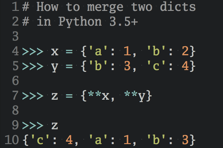


