Watch Now This tutorial has a related video course created by the Real Python team. Watch it together with the written tutorial to deepen your understanding: Introduction to Sorting Algorithms in Python
Sorting is a basic building block that many other algorithms are built upon. It’s related to several exciting ideas that you’ll see throughout your programming career. Understanding how sorting algorithms in Python work behind the scenes is a fundamental step toward implementing correct and efficient algorithms that solve real-world problems.
In this tutorial, you’ll learn:
- How different sorting algorithms in Python work and how they compare under different circumstances
- How Python’s built-in sort functionality works behind the scenes
- How different computer science concepts like recursion and divide and conquer apply to sorting
- How to measure the efficiency of an algorithm using Big O notation and Python’s
timeitmodule
By the end of this tutorial, you’ll understand sorting algorithms from both a theoretical and a practical standpoint. More importantly, you’ll have a deeper understanding of different algorithm design techniques that you can apply to other areas of your work. Let’s get started!
Free Download: Get a sample chapter from Python Tricks: The Book that shows you Python’s best practices with simple examples you can apply instantly to write more beautiful + Pythonic code.
The Importance of Sorting Algorithms in Python
Sorting is one of the most thoroughly studied algorithms in computer science. There are dozens of different sorting implementations and applications that you can use to make your code more efficient and effective.
You can use sorting to solve a wide range of problems:
-
Searching: Searching for an item on a list works much faster if the list is sorted.
-
Selection: Selecting items from a list based on their relationship to the rest of the items is easier with sorted data. For example, finding the kth-largest or smallest value, or finding the median value of the list, is much easier when the values are in ascending or descending order.
-
Duplicates: Finding duplicate values on a list can be done very quickly when the list is sorted.
-
Distribution: Analyzing the frequency distribution of items on a list is very fast if the list is sorted. For example, finding the element that appears most or least often is relatively straightforward with a sorted list.
From commercial applications to academic research and everywhere in between, there are countless ways you can use sorting to save yourself time and effort.
Python’s Built-In Sorting Algorithm
The Python language, like many other high-level programming languages, offers the ability to sort data out of the box using sorted(). Here’s an example of sorting an integer array:
>>> array = [8, 2, 6, 4, 5]
>>> sorted(array)
[2, 4, 5, 6, 8]
You can use sorted() to sort any list as long as the values inside are comparable.
Note: For a deeper dive into how Python’s built-in sorting functionality works, check out How to Use sorted() and .sort() in Python and Sorting Data With Python.
The Significance of Time Complexity
This tutorial covers two different ways to measure the runtime of sorting algorithms:
- For a practical point of view, you’ll measure the runtime of the implementations using the
timeitmodule. - For a more theoretical perspective, you’ll measure the runtime complexity of the algorithms using Big O notation.
Timing Your Code
When comparing two sorting algorithms in Python, it’s always informative to look at how long each one takes to run. The specific time each algorithm takes will be partly determined by your hardware, but you can still use the proportional time between executions to help you decide which implementation is more time efficient.
In this section, you’ll focus on a practical way to measure the actual time it takes to run to your sorting algorithms using the timeit module. For more information on the different ways you can time the execution of code in Python, check out Python Timer Functions: Three Ways to Monitor Your Code.
Here’s a function you can use to time your algorithms:
 1from random import randint
 2from timeit import repeat
 3
 4def run_sorting_algorithm(algorithm, array):
 5    # Set up the context and prepare the call to the specified
 6    # algorithm using the supplied array. Only import the
 7    # algorithm function if it's not the built-in `sorted()`.
 8    setup_code = f"from __main__ import {algorithm}" \
 9        if algorithm != "sorted" else ""
10
11    stmt = f"{algorithm}({array})"
12
13    # Execute the code ten different times and return the time
14    # in seconds that each execution took
15    times = repeat(setup=setup_code, stmt=stmt, repeat=3, number=10)
16
17    # Finally, display the name of the algorithm and the
18    # minimum time it took to run
19    print(f"Algorithm: {algorithm}. Minimum execution time: {min(times)}")
In this example, run_sorting_algorithm() receives the name of the algorithm and the input array that needs to be sorted. Here’s a line-by-line explanation of how it works:
-
Line 8 imports the name of the algorithm using the magic of Python’s f-strings. This is so that
timeit.repeat()knows where to call the algorithm from. Note that this is only necessary for the custom implementations used in this tutorial. If the algorithm specified is the built-insorted(), then nothing will be imported. -
Line 11 prepares the call to the algorithm with the supplied array. This is the statement that will be executed and timed.
-
Line 15 calls
timeit.repeat()with the setup code and the statement. This will call the specified sorting algorithm ten times, returning the number of seconds each one of these executions took. -
Line 19 identifies the shortest time returned and prints it along with the name of the algorithm.
Note: A common misconception is that you should find the average time of each run of the algorithm instead of selecting the single shortest time. Time measurements are noisy because the system runs other processes concurrently. The shortest time is always the least noisy, making it the best representation of the algorithm’s true runtime.
Here’s an example of how to use run_sorting_algorithm() to determine the time it takes to sort an array of ten thousand integer values using sorted():
21ARRAY_LENGTH = 10000
22
23if __name__ == "__main__":
24    # Generate an array of `ARRAY_LENGTH` items consisting
25    # of random integer values between 0 and 999
26    array = [randint(0, 1000) for i in range(ARRAY_LENGTH)]
27
28    # Call the function using the name of the sorting algorithm
29    # and the array you just created
30    run_sorting_algorithm(algorithm="sorted", array=array)
If you save the above code in a sorting.py file, then you can run it from the terminal and see its output:
$ python sorting.py
Algorithm: sorted. Minimum execution time: 0.010945824000000007
Remember that the time in seconds of every experiment depends in part on the hardware you use, so you’ll likely see slightly different results when running the code.
Note: You can learn more about the timeit module in the official Python documentation.
Measuring Efficiency With Big O Notation
The specific time an algorithm takes to run isn’t enough information to get the full picture of its time complexity. To solve this problem, you can use Big O (pronounced “big oh”) notation. Big O is often used to compare different implementations and decide which one is the most efficient, skipping unnecessary details and focusing on what’s most important in the runtime of an algorithm.
The time in seconds required to run different algorithms can be influenced by several unrelated factors, including processor speed or available memory. Big O, on the other hand, provides a platform to express runtime complexity in hardware-agnostic terms. With Big O, you express complexity in terms of how quickly your algorithm’s runtime grows relative to the size of the input, especially as the input grows arbitrarily large.
Assuming that n is the size of the input to an algorithm, the Big O notation represents the relationship between n and the number of steps the algorithm takes to find a solution. Big O uses a capital letter “O” followed by this relationship inside parentheses. For example, O(n) represents algorithms that execute a number of steps proportional to the size of their input.
Although this tutorial isn’t going to dive very deep into the details of Big O notation, here are five examples of the runtime complexity of different algorithms:
| Big O | Complexity | Description |
|---|---|---|
| O(1) | constant | The runtime is constant regardless of the size of the input. Finding an element in a hash table is an example of an operation that can be performed in constant time. |
| O(n) | linear | The runtime grows linearly with the size of the input. A function that checks a condition on every item of a list is an example of an O(n) algorithm. |
| O(n2) | quadratic | The runtime is a quadratic function of the size of the input. A naive implementation of finding duplicate values in a list, in which each item has to be checked twice, is an example of a quadratic algorithm. |
| O(2n) | exponential | The runtime grows exponentially with the size of the input. These algorithms are considered extremely inefficient. An example of an exponential algorithm is the three-coloring problem. |
| O(log n) | logarithmic | The runtime grows linearly while the size of the input grows exponentially. For example, if it takes one second to process one thousand elements, then it will take two seconds to process ten thousand, three seconds to process one hundred thousand, and so on. Binary search is an example of a logarithmic runtime algorithm. |
This tutorial covers the Big O runtime complexity of each of the sorting algorithms discussed. It also includes a brief explanation of how to determine the runtime on each particular case. This will give you a better understanding of how to start using Big O to classify other algorithms.
Note: For a deeper understanding of Big O, together with several practical examples in Python, check out Big O Notation and Algorithm Analysis with Python Examples.
The Bubble Sort Algorithm in Python
Bubble Sort is one of the most straightforward sorting algorithms. Its name comes from the way the algorithm works: With every new pass, the largest element in the list “bubbles up” toward its correct position.
Bubble sort consists of making multiple passes through a list, comparing elements one by one, and swapping adjacent items that are out of order.
Implementing Bubble Sort in Python
Here’s an implementation of a bubble sort algorithm in Python:
 1def bubble_sort(array):
 2    n = len(array)
 3
 4    for i in range(n):
 5        # Create a flag that will allow the function to
 6        # terminate early if there's nothing left to sort
 7        already_sorted = True
 8
 9        # Start looking at each item of the list one by one,
10        # comparing it with its adjacent value. With each
11        # iteration, the portion of the array that you look at
12        # shrinks because the remaining items have already been
13        # sorted.
14        for j in range(n - i - 1):
15            if array[j] > array[j + 1]:
16                # If the item you're looking at is greater than its
17                # adjacent value, then swap them
18                array[j], array[j + 1] = array[j + 1], array[j]
19
20                # Since you had to swap two elements,
21                # set the `already_sorted` flag to `False` so the
22                # algorithm doesn't finish prematurely
23                already_sorted = False
24
25        # If there were no swaps during the last iteration,
26        # the array is already sorted, and you can terminate
27        if already_sorted:
28            break
29
30    return array
Since this implementation sorts the array in ascending order, each step “bubbles” the largest element to the end of the array. This means that each iteration takes fewer steps than the previous iteration because a continuously larger portion of the array is sorted.
The loops in lines 4 and 10 determine the way the algorithm runs through the list. Notice how j initially goes from the first element in the list to the element immediately before the last. During the second iteration, j runs until two items from the last, then three items from the last, and so on. At the end of each iteration, the end portion of the list will be sorted.
As the loops progress, line 15 compares each element with its adjacent value, and line 18 swaps them if they are in the incorrect order. This ensures a sorted list at the end of the function.
Note: The already_sorted flag in lines 13, 23, and 27 of the code above is an optimization to the algorithm, and it’s not required in a fully functional bubble sort implementation. However, it allows the function to skip unnecessary steps if the list ends up wholly sorted before the loops have finished.
As an exercise, you can remove the use of this flag and compare the runtimes of both implementations.
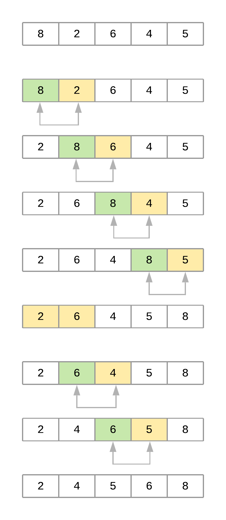
To properly analyze how the algorithm works, consider a list with values [8, 2, 6, 4, 5]. Assume you’re using bubble_sort() from above. Here’s a figure illustrating what the array looks like at each iteration of the algorithm:
Now take a step-by-step look at what’s happening with the array as the algorithm progresses:
-
The code starts by comparing the first element,
8, with its adjacent element,2. Since8 > 2, the values are swapped, resulting in the following order:[2, 8, 6, 4, 5]. -
The algorithm then compares the second element,
8, with its adjacent element,6. Since8 > 6, the values are swapped, resulting in the following order:[2, 6, 8, 4, 5]. -
Next, the algorithm compares the third element,
8, with its adjacent element,4. Since8 > 4, it swaps the values as well, resulting in the following order:[2, 6, 4, 8, 5]. -
Finally, the algorithm compares the fourth element,
8, with its adjacent element,5, and swaps them as well, resulting in[2, 6, 4, 5, 8]. At this point, the algorithm completed the first pass through the list (i = 0). Notice how the value8bubbled up from its initial location to its correct position at the end of the list. -
The second pass (
i = 1) takes into account that the last element of the list is already positioned and focuses on the remaining four elements,[2, 6, 4, 5]. At the end of this pass, the value6finds its correct position. The third pass through the list positions the value5, and so on until the list is sorted.
Measuring Bubble Sort’s Big O Runtime Complexity
Your implementation of bubble sort consists of two nested for loops in which the algorithm performs n - 1 comparisons, then n - 2 comparisons, and so on until the final comparison is done. This comes at a total of (n - 1) + (n - 2) + (n - 3) + … + 2 + 1 = n(n-1)/2 comparisons, which can also be written as ½n2 - ½n.
You learned earlier that Big O focuses on how the runtime grows in comparison to the size of the input. That means that, in order to turn the above equation into the Big O complexity of the algorithm, you need to remove the constants because they don’t change with the input size.
Doing so simplifies the notation to n2 - n. Since n2 grows much faster than n, this last term can be dropped as well, leaving bubble sort with an average- and worst-case complexity of O(n2).
In cases where the algorithm receives an array that’s already sorted—and assuming the implementation includes the already_sorted flag optimization explained before—the runtime complexity will come down to a much better O(n) because the algorithm will not need to visit any element more than once.
O(n), then, is the best-case runtime complexity of bubble sort. But keep in mind that best cases are an exception, and you should focus on the average case when comparing different algorithms.
Timing Your Bubble Sort Implementation
Using your run_sorting_algorithm() from earlier in this tutorial, here’s the time it takes for bubble sort to process an array with ten thousand items. Line 8 replaces the name of the algorithm and everything else stays the same:
 1if __name__ == "__main__":
 2    # Generate an array of `ARRAY_LENGTH` items consisting
 3    # of random integer values between 0 and 999
 4    array = [randint(0, 1000) for i in range(ARRAY_LENGTH)]
 5
 6    # Call the function using the name of the sorting algorithm
 7    # and the array you just created
 8    run_sorting_algorithm(algorithm="bubble_sort", array=array)
You can now run the script to get the execution time of bubble_sort:
$ python sorting.py
Algorithm: bubble_sort. Minimum execution time: 73.21720498399998
It took 73 seconds to sort the array with ten thousand elements. This represents the fastest execution out of the ten repetitions that run_sorting_algorithm() runs. Executing this script multiple times will produce similar results.
Note: A single execution of bubble sort took 73 seconds, but the algorithm ran ten times using timeit.repeat(). This means that you should expect your code to take around 73 * 10 = 730 seconds to run, assuming you have similar hardware characteristics. Slower machines may take much longer to finish.
Analyzing the Strengths and Weaknesses of Bubble Sort
The main advantage of the bubble sort algorithm is its simplicity. It is straightforward to both implement and understand. This is probably the main reason why most computer science courses introduce the topic of sorting using bubble sort.
As you saw before, the disadvantage of bubble sort is that it is slow, with a runtime complexity of O(n2). Unfortunately, this rules it out as a practical candidate for sorting large arrays.
The Insertion Sort Algorithm in Python
Like bubble sort, the insertion sort algorithm is straightforward to implement and understand. But unlike bubble sort, it builds the sorted list one element at a time by comparing each item with the rest of the list and inserting it into its correct position. This “insertion” procedure gives the algorithm its name.
An excellent analogy to explain insertion sort is the way you would sort a deck of cards. Imagine that you’re holding a group of cards in your hands, and you want to arrange them in order. You’d start by comparing a single card step by step with the rest of the cards until you find its correct position. At that point, you’d insert the card in the correct location and start over with a new card, repeating until all the cards in your hand were sorted.
Implementing Insertion Sort in Python
The insertion sort algorithm works exactly like the example with the deck of cards. Here’s the implementation in Python:
 1def insertion_sort(array):
 2    # Loop from the second element of the array until
 3    # the last element
 4    for i in range(1, len(array)):
 5        # This is the element we want to position in its
 6        # correct place
 7        key_item = array[i]
 8
 9        # Initialize the variable that will be used to
10        # find the correct position of the element referenced
11        # by `key_item`
12        j = i - 1
13
14        # Run through the list of items (the left
15        # portion of the array) and find the correct position
16        # of the element referenced by `key_item`. Do this only
17        # if `key_item` is smaller than its adjacent values.
18        while j >= 0 and array[j] > key_item:
19            # Shift the value one position to the left
20            # and reposition j to point to the next element
21            # (from right to left)
22            array[j + 1] = array[j]
23            j -= 1
24
25        # When you finish shifting the elements, you can position
26        # `key_item` in its correct location
27        array[j + 1] = key_item
28
29    return array
Unlike bubble sort, this implementation of insertion sort constructs the sorted list by pushing smaller items to the left. Let’s break down insertion_sort() line by line:
-
Line 4 sets up the loop that determines the
key_itemthat the function will position during each iteration. Notice that the loop starts with the second item on the list and goes all the way to the last item. -
Line 7 initializes
key_itemwith the item that the function is trying to place. -
Line 12 initializes a variable that will consecutively point to each element to the left of
key item. These are the elements that will be consecutively compared withkey_item. -
Line 18 compares
key_itemwith each value to its left using awhileloop, shifting the elements to make room to placekey_item. -
Line 27 positions
key_itemin its correct place after the algorithm shifts all the larger values to the right.
Here’s a figure illustrating the different iterations of the algorithm when sorting the array [8, 2, 6, 4, 5]:
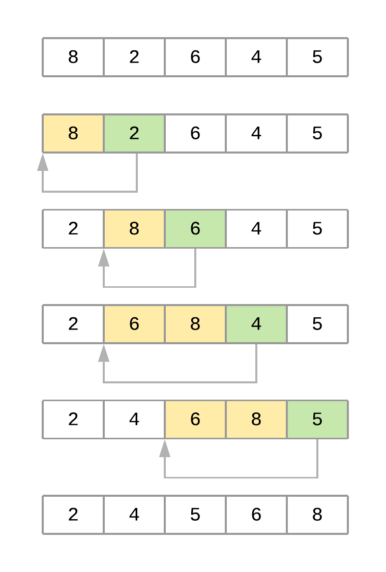
Now here’s a summary of the steps of the algorithm when sorting the array:
-
The algorithm starts with
key_item = 2and goes through the subarray to its left to find the correct position for it. In this case, the subarray is[8]. -
Since
2 < 8, the algorithm shifts element8one position to its right. The resultant array at this point is[8, 8, 6, 4, 5]. -
Since there are no more elements in the subarray, the
key_itemis now placed in its new position, and the final array is[2, 8, 6, 4, 5]. -
The second pass starts with
key_item = 6and goes through the subarray located to its left, in this case[2, 8]. -
Since
6 < 8, the algorithm shifts 8 to its right. The resultant array at this point is[2, 8, 8, 4, 5]. -
Since
6 > 2, the algorithm doesn’t need to keep going through the subarray, so it positionskey_itemand finishes the second pass. At this time, the resultant array is[2, 6, 8, 4, 5]. -
The third pass through the list puts the element
4in its correct position, and the fourth pass places element5in the correct spot, leaving the array sorted.
Measuring Insertion Sort’s Big O Runtime Complexity
Similar to your bubble sort implementation, the insertion sort algorithm has a couple of nested loops that go over the list. The inner loop is pretty efficient because it only goes through the list until it finds the correct position of an element. That said, the algorithm still has an O(n2) runtime complexity on the average case.
The worst case happens when the supplied array is sorted in reverse order. In this case, the inner loop has to execute every comparison to put every element in its correct position. This still gives you an O(n2) runtime complexity.
The best case happens when the supplied array is already sorted. Here, the inner loop is never executed, resulting in an O(n) runtime complexity, just like the best case of bubble sort.
Although bubble sort and insertion sort have the same Big O runtime complexity, in practice, insertion sort is considerably more efficient than bubble sort. If you look at the implementation of both algorithms, then you can see how insertion sort has to make fewer comparisons to sort the list.
Timing Your Insertion Sort Implementation
To prove the assertion that insertion sort is more efficient than bubble sort, you can time the insertion sort algorithm and compare it with the results of bubble sort. To do this, you just need to replace the call to run_sorting_algorithm() with the name of your insertion sort implementation:
 1if __name__ == "__main__":
 2    # Generate an array of `ARRAY_LENGTH` items consisting
 3    # of random integer values between 0 and 999
 4    array = [randint(0, 1000) for i in range(ARRAY_LENGTH)]
 5
 6    # Call the function using the name of the sorting algorithm
 7    # and the array we just created
 8    run_sorting_algorithm(algorithm="insertion_sort", array=array)
You can execute the script as before:
$ python sorting.py
Algorithm: insertion_sort. Minimum execution time: 56.71029764299999
Notice how the insertion sort implementation took around 17 fewer seconds than the bubble sort implementation to sort the same array. Even though they’re both O(n2) algorithms, insertion sort is more efficient.
Analyzing the Strengths and Weaknesses of Insertion Sort
Just like bubble sort, the insertion sort algorithm is very uncomplicated to implement. Even though insertion sort is an O(n2) algorithm, it’s also much more efficient in practice than other quadratic implementations such as bubble sort.
There are more powerful algorithms, including merge sort and Quicksort, but these implementations are recursive and usually fail to beat insertion sort when working on small lists. Some Quicksort implementations even use insertion sort internally if the list is small enough to provide a faster overall implementation. Timsort also uses insertion sort internally to sort small portions of the input array.
That said, insertion sort is not practical for large arrays, opening the door to algorithms that can scale in more efficient ways.
The Merge Sort Algorithm in Python
Merge sort is a very efficient sorting algorithm. It’s based on the divide-and-conquer approach, a powerful algorithmic technique used to solve complex problems.
To properly understand divide and conquer, you should first understand the concept of recursion. Recursion involves breaking a problem down into smaller subproblems until they’re small enough to manage. In programming, recursion is usually expressed by a function calling itself.
Note: This tutorial doesn’t explore recursion in depth. To better understand how recursion works and see it in action using Python, check out Thinking Recursively in Python and Recursion in Python: An Introduction.
Divide-and-conquer algorithms typically follow the same structure:
- The original input is broken into several parts, each one representing a subproblem that’s similar to the original but simpler.
- Each subproblem is solved recursively.
- The solutions to all the subproblems are combined into a single overall solution.
In the case of merge sort, the divide-and-conquer approach divides the set of input values into two equal-sized parts, sorts each half recursively, and finally merges these two sorted parts into a single sorted list.
Implementing Merge Sort in Python
The implementation of the merge sort algorithm needs two different pieces:
- A function that recursively splits the input in half
- A function that merges both halves, producing a sorted array
Here’s the code to merge two different arrays:
 1def merge(left, right):
 2    # If the first array is empty, then nothing needs
 3    # to be merged, and you can return the second array as the result
 4    if len(left) == 0:
 5        return right
 6
 7    # If the second array is empty, then nothing needs
 8    # to be merged, and you can return the first array as the result
 9    if len(right) == 0:
10        return left
11
12    result = []
13    index_left = index_right = 0
14
15    # Now go through both arrays until all the elements
16    # make it into the resultant array
17    while len(result) < len(left) + len(right):
18        # The elements need to be sorted to add them to the
19        # resultant array, so you need to decide whether to get
20        # the next element from the first or the second array
21        if left[index_left] <= right[index_right]:
22            result.append(left[index_left])
23            index_left += 1
24        else:
25            result.append(right[index_right])
26            index_right += 1
27
28        # If you reach the end of either array, then you can
29        # add the remaining elements from the other array to
30        # the result and break the loop
31        if index_right == len(right):
32            result += left[index_left:]
33            break
34
35        if index_left == len(left):
36            result += right[index_right:]
37            break
38
39    return result
merge() receives two different sorted arrays that need to be merged together. The process to accomplish this is straightforward:
-
Lines 4 and 9 check whether either of the arrays is empty. If one of them is, then there’s nothing to merge, so the function returns the other array.
-
Line 17 starts a
whileloop that ends whenever the result contains all the elements from both of the supplied arrays. The goal is to look into both arrays and combine their items to produce a sorted list. -
Line 21 compares the elements at the head of both arrays, selects the smaller value, and appends it to the end of the resultant array.
-
Lines 31 and 35 append any remaining items to the result if all the elements from either of the arrays were already used.
With the above function in place, the only missing piece is a function that recursively splits the input array in half and uses merge() to produce the final result:
41def merge_sort(array):
42    # If the input array contains fewer than two elements,
43    # then return it as the result of the function
44    if len(array) < 2:
45        return array
46
47    midpoint = len(array) // 2
48
49    # Sort the array by recursively splitting the input
50    # into two equal halves, sorting each half and merging them
51    # together into the final result
52    return merge(
53        left=merge_sort(array[:midpoint]),
54        right=merge_sort(array[midpoint:]))
Here’s a quick summary of the code:
-
Line 44 acts as the stopping condition for the recursion. If the input array contains fewer than two elements, then the function returns the array. Notice that this condition could be triggered by receiving either a single item or an empty array. In both cases, there’s nothing left to sort, so the function should return.
-
Line 47 computes the middle point of the array.
-
Line 52 calls
merge(), passing both sorted halves as the arrays.
Notice how this function calls itself recursively, halving the array each time. Each iteration deals with an ever-shrinking array until fewer than two elements remain, meaning there’s nothing left to sort. At this point, merge() takes over, merging the two halves and producing a sorted list.
Take a look at a representation of the steps that merge sort will take to sort the array [8, 2, 6, 4, 5]:
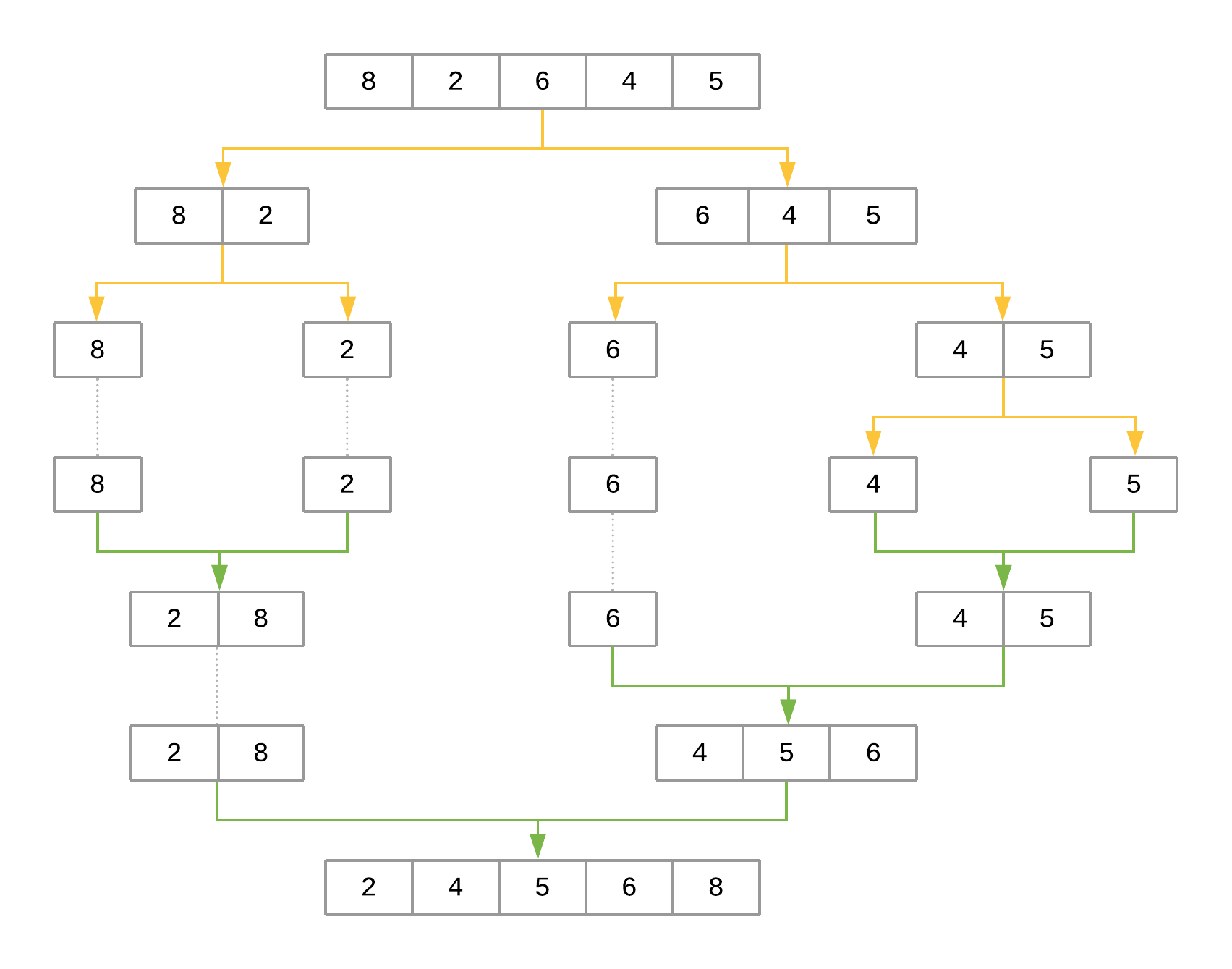
The figure uses yellow arrows to represent halving the array at each recursion level. The green arrows represent merging each subarray back together. The steps can be summarized as follows:
-
The first call to
merge_sort()with[8, 2, 6, 4, 5]definesmidpointas2. Themidpointis used to halve the input array intoarray[:2]andarray[2:], producing[8, 2]and[6, 4, 5], respectively.merge_sort()is then recursively called for each half to sort them separately. -
The call to
merge_sort()with[8, 2]produces[8]and[2]. The process repeats for each of these halves. -
The call to
merge_sort()with[8]returns[8]since that’s the only element. The same happens with the call tomerge_sort()with[2]. -
At this point, the function starts merging the subarrays back together using
merge(), starting with[8]and[2]as input arrays, producing[2, 8]as the result. -
On the other side,
[6, 4, 5]is recursively broken down and merged using the same procedure, producing[4, 5, 6]as the result. -
In the final step,
[2, 8]and[4, 5, 6]are merged back together withmerge(), producing the final result:[2, 4, 5, 6, 8].
Measuring Merge Sort’s Big O Complexity
To analyze the complexity of merge sort, you can look at its two steps separately:
-
merge()has a linear runtime. It receives two arrays whose combined length is at most n (the length of the original input array), and it combines both arrays by looking at each element at most once. This leads to a runtime complexity of O(n). -
The second step splits the input array recursively and calls
merge()for each half. Since the array is halved until a single element remains, the total number of halving operations performed by this function is log2n. Sincemerge()is called for each half, we get a total runtime of O(n log2n).
Interestingly, O(n log2n) is the best possible worst-case runtime that can be achieved by a sorting algorithm.
Timing Your Merge Sort Implementation
To compare the speed of merge sort with the previous two implementations, you can use the same mechanism as before and replace the name of the algorithm in line 8:
 1if __name__ == "__main__":
 2    # Generate an array of `ARRAY_LENGTH` items consisting
 3    # of random integer values between 0 and 999
 4    array = [randint(0, 1000) for i in range(ARRAY_LENGTH)]
 5
 6    # Call the function using the name of the sorting algorithm
 7    # and the array you just created
 8    run_sorting_algorithm(algorithm="merge_sort", array=array)
You can execute the script to get the execution time of merge_sort:
$ python sorting.py
Algorithm: merge_sort. Minimum execution time: 0.6195857160000173
Compared to bubble sort and insertion sort, the merge sort implementation is extremely fast, sorting the ten-thousand-element array in less than a second!
Analyzing the Strengths and Weaknesses of Merge Sort
Thanks to its runtime complexity of O(n log2n), merge sort is a very efficient algorithm that scales well as the size of the input array grows. It’s also straightforward to parallelize because it breaks the input array into chunks that can be distributed and processed in parallel if necessary.
That said, for small lists, the time cost of the recursion allows algorithms such as bubble sort and insertion sort to be faster. For example, running an experiment with a list of ten elements results in the following times:
Algorithm: bubble_sort. Minimum execution time: 0.000018774999999998654
Algorithm: insertion_sort. Minimum execution time: 0.000029786000000000395
Algorithm: merge_sort. Minimum execution time: 0.00016983000000000276
Both bubble sort and insertion sort beat merge sort when sorting a ten-element list.
Another drawback of merge sort is that it creates copies of the array when calling itself recursively. It also creates a new list inside merge() to sort and return both input halves. This makes merge sort use much more memory than bubble sort and insertion sort, which are both able to sort the list in place.
Due to this limitation, you may not want to use merge sort to sort large lists in memory-constrained hardware.
The Quicksort Algorithm in Python
Just like merge sort, the Quicksort algorithm applies the divide-and-conquer principle to divide the input array into two lists, the first with small items and the second with large items. The algorithm then sorts both lists recursively until the resultant list is completely sorted.
Dividing the input list is referred to as partitioning the list. Quicksort first selects a pivot element and partitions the list around the pivot, putting every smaller element into a low array and every larger element into a high array.
Putting every element from the low list to the left of the pivot and every element from the high list to the right positions the pivot precisely where it needs to be in the final sorted list. This means that the function can now recursively apply the same procedure to low and then high until the entire list is sorted.
Implementing Quicksort in Python
Here’s a fairly compact implementation of Quicksort:
 1from random import randint
 2
 3def quicksort(array):
 4    # If the input array contains fewer than two elements,
 5    # then return it as the result of the function
 6    if len(array) < 2:
 7        return array
 8
 9    low, same, high = [], [], []
10
11    # Select your `pivot` element randomly
12    pivot = array[randint(0, len(array) - 1)]
13
14    for item in array:
15        # Elements that are smaller than the `pivot` go to
16        # the `low` list. Elements that are larger than
17        # `pivot` go to the `high` list. Elements that are
18        # equal to `pivot` go to the `same` list.
19        if item < pivot:
20            low.append(item)
21        elif item == pivot:
22            same.append(item)
23        elif item > pivot:
24            high.append(item)
25
26    # The final result combines the sorted `low` list
27    # with the `same` list and the sorted `high` list
28    return quicksort(low) + same + quicksort(high)
Here’s a summary of the code:
-
Line 6 stops the recursive function if the array contains fewer than two elements.
-
Line 12 selects the
pivotelement randomly from the list and proceeds to partition the list. -
Lines 19 and 20 put every element that’s smaller than
pivotinto the list calledlow. -
Lines 21 and 22 put every element that’s equal to
pivotinto the list calledsame. -
Lines 23 and 24 put every element that’s larger than
pivotinto the list calledhigh. -
Line 28 recursively sorts the
lowandhighlists and combines them along with the contents of thesamelist.
Here’s an illustration of the steps that Quicksort takes to sort the array [8, 2, 6, 4, 5]:
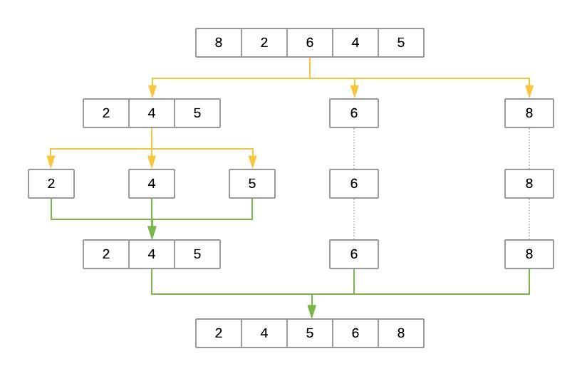
The yellow lines represent the partitioning of the array into three lists: low, same, and high. The green lines represent sorting and putting these lists back together. Here’s a brief explanation of the steps:
-
The
pivotelement is selected randomly. In this case,pivotis6. -
The first pass partitions the input array so that
lowcontains[2, 4, 5],samecontains[6], andhighcontains[8]. -
quicksort()is then called recursively withlowas its input. This selects a randompivotand breaks the array into[2]aslow,[4]assame, and[5]ashigh. -
The process continues, but at this point, both
lowandhighhave fewer than two items each. This ends the recursion, and the function puts the array back together. Adding the sortedlowandhighto either side of thesamelist produces[2, 4, 5]. -
On the other side, the
highlist containing[8]has fewer than two elements, so the algorithm returns the sortedlowarray, which is now[2, 4, 5]. Merging it withsame([6]) andhigh([8]) produces the final sorted list.
Selecting the pivot Element
Why does the implementation above select the pivot element randomly? Wouldn’t it be the same to consistently select the first or last element of the input list?
Because of how the Quicksort algorithm works, the number of recursion levels depends on where pivot ends up in each partition. In the best-case scenario, the algorithm consistently picks the median element as the pivot. That would make each generated subproblem exactly half the size of the previous problem, leading to at most log2n levels.
On the other hand, if the algorithm consistently picks either the smallest or largest element of the array as the pivot, then the generated partitions will be as unequal as possible, leading to n-1 recursion levels. That would be the worst-case scenario for Quicksort.
As you can see, Quicksort’s efficiency often depends on the pivot selection. If the input array is unsorted, then using the first or last element as the pivot will work the same as a random element. But if the input array is sorted or almost sorted, using the first or last element as the pivot could lead to a worst-case scenario. Selecting the pivot at random makes it more likely Quicksort will select a value closer to the median and finish faster.
Another option for selecting the pivot is to find the median value of the array and force the algorithm to use it as the pivot. This can be done in O(n) time. Although the process is little bit more involved, using the median value as the pivot for Quicksort guarantees you will have the best-case Big O scenario.
Measuring Quicksort’s Big O Complexity
With Quicksort, the input list is partitioned in linear time, O(n), and this process repeats recursively an average of log2n times. This leads to a final complexity of O(n log2n).
That said, remember the discussion about how the selection of the pivot affects the runtime of the algorithm. The O(n) best-case scenario happens when the selected pivot is close to the median of the array, and an O(n2) scenario happens when the pivot is the smallest or largest value of the array.
Theoretically, if the algorithm focuses first on finding the median value and then uses it as the pivot element, then the worst-case complexity will come down to O(n log2n). The median of an array can be found in linear time, and using it as the pivot guarantees the Quicksort portion of the code will perform in O(n log2n).
By using the median value as the pivot, you end up with a final runtime of O(n) + O(n log2n). You can simplify this down to O(n log2n) because the logarithmic portion grows much faster than the linear portion.
Note: Although achieving O(n log2n) is possible in Quicksort’s worst-case scenario, this approach is seldom used in practice. Lists have to be quite large for the implementation to be faster than a simple randomized selection of the pivot.
Randomly selecting the pivot makes the worst case very unlikely. That makes random pivot selection good enough for most implementations of the algorithm.
Timing Your Quicksort Implementation
By now, you’re familiar with the process for timing the runtime of the algorithm. Just change the name of the algorithm in line 8:
 1if __name__ == "__main__":
 2    # Generate an array of `ARRAY_LENGTH` items consisting
 3    # of random integer values between 0 and 999
 4    array = [randint(0, 1000) for i in range(ARRAY_LENGTH)]
 5
 6    # Call the function using the name of the sorting algorithm
 7    # and the array you just created
 8    run_sorting_algorithm(algorithm="quicksort", array=array)
You can execute the script as you have before:
$ python sorting.py
Algorithm: quicksort. Minimum execution time: 0.11675417600002902
Not only does Quicksort finish in less than one second, but it’s also much faster than merge sort (0.11 seconds versus 0.61 seconds). Increasing the number of elements specified by ARRAY_LENGTH from 10,000 to 1,000,000 and running the script again ends up with merge sort finishing in 97 seconds, whereas Quicksort sorts the list in a mere 10 seconds.
Analyzing the Strengths and Weaknesses of Quicksort
True to its name, Quicksort is very fast. Although its worst-case scenario is theoretically O(n2), in practice, a good implementation of Quicksort beats most other sorting implementations. Also, just like merge sort, Quicksort is straightforward to parallelize.
One of Quicksort’s main disadvantages is the lack of a guarantee that it will achieve the average runtime complexity. Although worst-case scenarios are rare, certain applications can’t afford to risk poor performance, so they opt for algorithms that stay within O(n log2n) regardless of the input.
Just like merge sort, Quicksort also trades off memory space for speed. This may become a limitation for sorting larger lists.
A quick experiment sorting a list of ten elements leads to the following results:
Algorithm: bubble_sort. Minimum execution time: 0.0000909000000000014
Algorithm: insertion_sort. Minimum execution time: 0.00006681900000000268
Algorithm: quicksort. Minimum execution time: 0.0001319930000000004
The results show that Quicksort also pays the price of recursion when the list is sufficiently small, taking longer to complete than both insertion sort and bubble sort.
The Timsort Algorithm in Python
The Timsort algorithm is considered a hybrid sorting algorithm because it employs a best-of-both-worlds combination of insertion sort and merge sort. Timsort is near and dear to the Python community because it was created by Tim Peters in 2002 to be used as the standard sorting algorithm of the Python language.
The main characteristic of Timsort is that it takes advantage of already-sorted elements that exist in most real-world datasets. These are called natural runs. The algorithm then iterates over the list, collecting the elements into runs and merging them into a single sorted list.
Implementing Timsort in Python
In this section, you’ll create a barebones Python implementation that illustrates all the pieces of the Timsort algorithm. If you’re interested, you can also check out the original C implementation of Timsort.
The first step in implementing Timsort is modifying the implementation of insertion_sort() from before:
 1def insertion_sort(array, left=0, right=None):
 2    if right is None:
 3        right = len(array) - 1
 4
 5    # Loop from the element indicated by
 6    # `left` until the element indicated by `right`
 7    for i in range(left + 1, right + 1):
 8        # This is the element we want to position in its
 9        # correct place
10        key_item = array[i]
11
12        # Initialize the variable that will be used to
13        # find the correct position of the element referenced
14        # by `key_item`
15        j = i - 1
16
17        # Run through the list of items (the left
18        # portion of the array) and find the correct position
19        # of the element referenced by `key_item`. Do this only
20        # if the `key_item` is smaller than its adjacent values.
21        while j >= left and array[j] > key_item:
22            # Shift the value one position to the left
23            # and reposition `j` to point to the next element
24            # (from right to left)
25            array[j + 1] = array[j]
26            j -= 1
27
28        # When you finish shifting the elements, position
29        # the `key_item` in its correct location
30        array[j + 1] = key_item
31
32    return array
This modified implementation adds a couple of parameters, left and right, that indicate which portion of the array should be sorted. This allows the Timsort algorithm to sort a portion of the array in place. Modifying the function instead of creating a new one means that it can be reused for both insertion sort and Timsort.
Now take a look at the implementation of Timsort:
 1def timsort(array):
 2    min_run = 32
 3    n = len(array)
 4
 5    # Start by slicing and sorting small portions of the
 6    # input array. The size of these slices is defined by
 7    # your `min_run` size.
 8    for i in range(0, n, min_run):
 9        insertion_sort(array, i, min((i + min_run - 1), n - 1))
10
11    # Now you can start merging the sorted slices.
12    # Start from `min_run`, doubling the size on
13    # each iteration until you surpass the length of
14    # the array.
15    size = min_run
16    while size < n:
17        # Determine the arrays that will
18        # be merged together
19        for start in range(0, n, size * 2):
20            # Compute the `midpoint` (where the first array ends
21            # and the second starts) and the `endpoint` (where
22            # the second array ends)
23            midpoint = start + size - 1
24            end = min((start + size * 2 - 1), (n-1))
25
26            # Merge the two subarrays.
27            # The `left` array should go from `start` to
28            # `midpoint + 1`, while the `right` array should
29            # go from `midpoint + 1` to `end + 1`.
30            merged_array = merge(
31                left=array[start:midpoint + 1],
32                right=array[midpoint + 1:end + 1])
33
34            # Finally, put the merged array back into
35            # your array
36            array[start:start + len(merged_array)] = merged_array
37
38        # Each iteration should double the size of your arrays
39        size *= 2
40
41    return array
Although the implementation is a bit more complex than the previous algorithms, we can summarize it quickly in the following way:
-
Lines 8 and 9 create small slices, or runs, of the array and sort them using insertion sort. You learned previously that insertion sort is speedy on small lists, and Timsort takes advantage of this. Timsort uses the newly introduced
leftandrightparameters ininsertion_sort()to sort the list in place without having to create new arrays like merge sort and Quicksort do. -
Line 16 merges these smaller runs, with each run being of size
32initially. With each iteration, the size of the runs is doubled, and the algorithm continues merging these larger runs until a single sorted run remains.
Notice how, unlike merge sort, Timsort merges subarrays that were previously sorted. Doing so decreases the total number of comparisons required to produce a sorted list. This advantage over merge sort will become apparent when running experiments using different arrays.
Finally, line 2 defines min_run = 32. There are two reasons for using 32 as the value here:
-
Sorting small arrays using insertion sort is very fast, and
min_runhas a small value to take advantage of this characteristic. Initializingmin_runwith a value that’s too large will defeat the purpose of using insertion sort and will make the algorithm slower. -
Merging two balanced lists is much more efficient than merging lists of disproportionate size. Picking a
min_runvalue that’s a power of two ensures better performance when merging all the different runs that the algorithm creates.
Combining both conditions above offers several options for min_run. The implementation in this tutorial uses min_run = 32 as one of the possibilities.
Note: In practice, Timsort does something a little more complicated to compute min_run. It picks a value between 32 and 64 inclusive, such that the length of the list divided by min_run is exactly a power of 2. If that’s not possible, it chooses a value that’s close to, but strictly less than, a power of 2.
If you’re curious, you can read the complete analysis on how to pick min_run under the Computing minrun section.
Measuring Timsort’s Big O Complexity
On average, the complexity of Timsort is O(n log2n), just like merge sort and Quicksort. The logarithmic part comes from doubling the size of the run to perform each linear merge operation.
However, Timsort performs exceptionally well on already-sorted or close-to-sorted lists, leading to a best-case scenario of O(n). In this case, Timsort clearly beats merge sort and matches the best-case scenario for Quicksort. But the worst case for Timsort is also O(n log2n), which surpasses Quicksort’s O(n2).
Timing Your Timsort Implementation
You can use run_sorting_algorithm() to see how Timsort performs sorting the ten-thousand-element array:
 1if __name__ == "__main__":
 2    # Generate an array of `ARRAY_LENGTH` items consisting
 3    # of random integer values between 0 and 999
 4    array = [randint(0, 1000) for i in range(ARRAY_LENGTH)]
 5
 6    # Call the function using the name of the sorting algorithm
 7    # and the array you just created
 8    run_sorting_algorithm(algorithm="timsort", array=array)
Now execute the script to get the execution time of timsort:
$ python sorting.py
Algorithm: timsort. Minimum execution time: 0.5121690789999998
At 0.51 seconds, this Timsort implementation is a full 0.1 seconds, or 17 percent, faster than merge sort, though it doesn’t match the 0.11 of Quicksort. It’s also a ridiculous 11,000 percent faster than insertion sort!
Now try to sort an already-sorted list using these four algorithms and see what happens. You can modify your __main__ section as follows:
 1if __name__ == "__main__":
 2    # Generate a sorted array of ARRAY_LENGTH items
 3    array = [i for i in range(ARRAY_LENGTH)]
 4
 5    # Call each of the functions
 6    run_sorting_algorithm(algorithm="insertion_sort", array=array)
 7    run_sorting_algorithm(algorithm="merge_sort", array=array)
 8    run_sorting_algorithm(algorithm="quicksort", array=array)
 9    run_sorting_algorithm(algorithm="timsort", array=array)
If you execute the script now, then all the algorithms will run and output their corresponding execution time:
Algorithm: insertion_sort. Minimum execution time: 53.5485634999991
Algorithm: merge_sort. Minimum execution time: 0.372304601
Algorithm: quicksort. Minimum execution time: 0.24626494199999982
Algorithm: timsort. Minimum execution time: 0.23350277099999994
This time, Timsort comes in at a whopping thirty-seven percent faster than merge sort and five percent faster than Quicksort, flexing its ability to take advantage of the already-sorted runs.
Notice how Timsort benefits from two algorithms that are much slower when used by themselves. The genius of Timsort is in combining these algorithms and playing to their strengths to achieve impressive results.
Analyzing the Strengths and Weaknesses of Timsort
The main disadvantage of Timsort is its complexity. Despite implementing a very simplified version of the original algorithm, it still requires much more code because it relies on both insertion_sort() and merge().
One of Timsort’s advantages is its ability to predictably perform in O(n log2n) regardless of the structure of the input array. Contrast that with Quicksort, which can degrade down to O(n2). Timsort is also very fast for small arrays because the algorithm turns into a single insertion sort.
For real-world usage, in which it’s common to sort arrays that already have some preexisting order, Timsort is a great option. Its adaptability makes it an excellent choice for sorting arrays of any length.
Conclusion
Sorting is an essential tool in any Pythonista’s toolkit. With knowledge of the different sorting algorithms in Python and how to maximize their potential, you’re ready to implement faster, more efficient apps and programs!
In this tutorial, you learned:
- How Python’s built-in
sort()works behind the scenes - What Big O notation is and how to use it to compare the efficiency of different algorithms
- How to measure the actual time spent running your code
- How to implement five different sorting algorithms in Python
- What the pros and cons are of using different algorithms
You also learned about different techniques such as recursion, divide and conquer, and randomization. These are fundamental building blocks for solving a long list of different algorithms, and they’ll come up again and again as you keep researching.
Take the code presented in this tutorial, create new experiments, and explore these algorithms further. Better yet, try implementing other sorting algorithms in Python. The list is vast, but selection sort, heapsort, and tree sort are three excellent options to start with.
Watch Now This tutorial has a related video course created by the Real Python team. Watch it together with the written tutorial to deepen your understanding: Introduction to Sorting Algorithms in Python