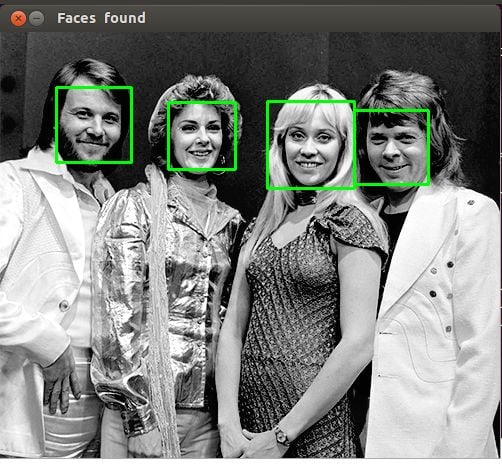
Why would you want to know more about different ways of storing and accessing images in Python? If you’re segmenting a handful of images by color or detecting faces one by one using OpenCV, then you don’t need to worry about it. Even if you’re using the Python Imaging Library (PIL) to draw on a few hundred photos, you still don’t need to. Storing images on disk, as .png or .jpg files, is both suitable and appropriate.
Increasingly, however, the number of images required for a given task is getting larger and larger. Algorithms like convolutional neural networks, also known as convnets or CNNs, can handle enormous datasets of images and even learn from them. If you’re interested, you can read more about how convnets can be used for ranking selfies or for sentiment analysis.
ImageNet is a well-known public image database put together for training models on tasks like object classification, detection, and segmentation, and it consists of over 14 million images.
Think about how long it would take to load all of them into memory for training, in batches, perhaps hundreds or thousands of times. Keep reading, and you’ll be convinced that it would take quite awhile—at least long enough to leave your computer and do many other things while you wish you worked at Google or NVIDIA.
In this tutorial, you’ll learn about:
- Storing images on disk as
.pngfiles - Storing images in lightning memory-mapped databases (LMDB)
- Storing images in hierarchical data format (HDF5)
You’ll also explore the following:
- Why alternate storage methods are worth considering
- What the performance differences are when you’re reading and writing single images
- What the performance differences are when you’re reading and writing many images
- How the three methods compare in terms of disk usage
If none of the storage methods ring a bell, don’t worry: for this article, all you need is a reasonably solid foundation in Python and a basic understanding of images (that they are really composed of multi-dimensional arrays of numbers) and relative memory, such as the difference between 10MB and 10GB.
Let’s get started!
Free Bonus: Click here to get the Python Face Detection & OpenCV Examples Mini-Guide that shows you practical code examples of real-world Python computer vision techniques.
Setup
You will need an image dataset to experiment with, as well as a few Python packages.
A Dataset to Play With
We will be using the Canadian Institute for Advanced Research image dataset, better known as CIFAR-10, which consists of 60,000 32x32 pixel color images belonging to different object classes, such as dogs, cats, and airplanes. Relatively, CIFAR is not a very large dataset, but if we were to use the full TinyImages dataset, then you would need about 400GB of free disk space, which would probably be a limiting factor.
Credits for the dataset as described in chapter 3 of this tech report go to Alex Krizhevsky, Vinod Nair, and Geoffrey Hinton.
If you’d like to follow along with the code examples in this article, you can download CIFAR-10 here, selecting the Python version. You’ll be sacrificing 163MB of disk space:

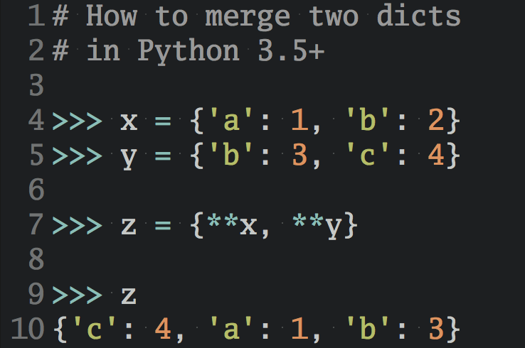
When you download and unzip the folder, you’ll discover that the files are not human-readable image files. They have actually been serialized and saved in batches using cPickle.
While we won’t consider pickle or cPickle in this article, other than to extract the CIFAR dataset, it’s worth mentioning that the Python pickle module has the key advantage of being able to serialize any Python object without any extra code or transformation on your part. It also has a potentially serious disadvantage of posing a security risk and not coping well when dealing with very large quantities of data.
The following code unpickles each of the five batch files and loads all of the images into a NumPy array:
import numpy as np
import pickle
from pathlib import Path

# Path to the unzipped CIFAR data
data_dir = Path("data/cifar-10-batches-py/")

# Unpickle function provided by the CIFAR hosts
def unpickle(file):
    with open(file, "rb") as fo:
        dict = pickle.load(fo, encoding="bytes")
    return dict

images, labels = [], []
for batch in data_dir.glob("data_batch_*"):
    batch_data = unpickle(batch)
    for i, flat_im in enumerate(batch_data[b"data"]):
        im_channels = []
        # Each image is flattened, with channels in order of R, G, B
        for j in range(3):
            im_channels.append(
                flat_im[j * 1024 : (j + 1) * 1024].reshape((32, 32))
            )
        # Reconstruct the original image
        images.append(np.dstack((im_channels)))
        # Save the label
        labels.append(batch_data[b"labels"][i])

print("Loaded CIFAR-10 training set:")
print(f" - np.shape(images)     {np.shape(images)}")
print(f" - np.shape(labels)     {np.shape(labels)}")
All the images are now in RAM in the images variable, with their corresponding meta data in labels, and are ready for you to manipulate. Next, you can install the Python packages you’ll use for the three methods.
Note: That last code block used f-strings. You can read more about them in Python’s F-String for String Interpolation and Formatting.
Setup for Storing Images on Disk
You’ll need to set up your environment for the default method of saving and accessing these images from disk. This article will assume you have Python 3.x installed on your system, and will use Pillow for the image manipulation:
$ pip install Pillow
Alternatively, if you prefer, you can install it using Anaconda:
$ conda install -c conda-forge pillow
Note: PIL is the original version of the Python Imaging Library, which is no longer maintained and is not compatible with Python 3.x. If you have previously installed PIL, make sure to uninstall it before installing Pillow, as they can’t exist together.
Now you’re ready for storing and reading images from disk.
Getting Started With LMDB
LMDB, sometimes referred to as the “Lightning Database,” stands for Lightning Memory-Mapped Database because it’s fast and uses memory-mapped files. It’s a key-value store, not a relational database.
In terms of implementation, LMDB is a B+ tree, which basically means that it is a tree-like graph structure stored in memory where each key-value element is a node, and nodes can have many children. Nodes on the same level are linked to one another for fast traversal.
Critically, key components of the B+ tree are set to correspond to the page size of the host operating system, maximizing efficiency when accessing any key-value pair in the database. Since LMDB high-performance heavily relies on this particular point, LMDB efficiency has been shown to be dependent on the underlying file system and its implementation.
Another key reason for the efficiency of LMDB is that it is memory-mapped. This means that it returns direct pointers to the memory addresses of both keys and values, without needing to copy anything in memory as most other databases do.
Those who want to dive into a bit more of the internal implementation details of B+ trees can check out this article on B+ trees and then play with this visualization of node insertion.
If B+ trees don’t interest you, don’t worry. You don’t need to know much about their internal implementation in order to use LMDB. We will be using the Python binding for the LMDB C library, which can be installed via pip:
$ pip install lmdb
You also have the option of installing via Anaconda:
$ conda install -c conda-forge python-lmdb
Check that you can import lmdb from a Python shell, and you’re good to go.
Getting Started With HDF5
HDF5 stands for Hierarchical Data Format, a file format referred to as HDF4 or HDF5. We don’t need to worry about HDF4, as HDF5 is the current maintained version.
Interestingly, HDF has its origins in the National Center for Supercomputing Applications, as a portable, compact scientific data format. If you’re wondering if it’s widely used, check out NASA’s blurb on HDF5 from their Earth Data project.
HDF files consist of two types of objects:
- Datasets
- Groups
Datasets are multidimensional arrays, and groups consist of datasets or other groups. Multidimensional arrays of any size and type can be stored as a dataset, but the dimensions and type have to be uniform within a dataset. Each dataset must contain a homogeneous N-dimensional array. That said, because groups and datasets may be nested, you can still get the heterogeneity you may need:
$ pip install h5py
As with the other libraries, you can alternately install via Anaconda:
$ conda install -c conda-forge h5py
If you can import h5py from a Python shell, everything is set up properly.
Storing a Single Image
Now that you have a general overview of the methods, let’s dive straight in and look at a quantitative comparison of the basic tasks we care about: how long it takes to read and write files, and how much disk memory will be used. This will also serve as a basic introduction to how the methods work, with code examples of how to use them.
When I refer to “files,” I generally mean a lot of them. However, it is important to make a distinction since some methods may be optimized for different operations and quantities of files.
For the purposes of experimentation, we can compare the performance between various quantities of files, by factors of 10 from a single image to 100,000 images. Since our five batches of CIFAR-10 add up to 50,000 images, we can use each image twice to get to 100,000 images.
To prepare for the experiments, you will want to create a folder for each method, which will contain all the database files or images, and save the paths to those directories in variables:
from pathlib import Path

disk_dir = Path("data/disk/")
lmdb_dir = Path("data/lmdb/")
hdf5_dir = Path("data/hdf5/")
Path does not automatically create the folders for you unless you specifically ask it to:
disk_dir.mkdir(parents=True, exist_ok=True)
lmdb_dir.mkdir(parents=True, exist_ok=True)
hdf5_dir.mkdir(parents=True, exist_ok=True)
Now you can move on to running the actual experiments, with code examples of how to perform basic tasks with the three different methods. We can use the timeit module, which is included in the Python standard library, to help time the experiments.
Although the main purpose of this article is not to learn the APIs of the different Python packages, it is helpful to have an understanding of how they can be implemented. We will go through the general principles alongside all the code used to conduct the storing experiments.
Storing to Disk
Our input for this experiment is a single image image, currently in memory as a NumPy array. You want to save it first to disk as a .png image, and name it using a unique image ID image_id. This can be done using the Pillow package you installed earlier:
from PIL import Image
import csv

def store_single_disk(image, image_id, label):
    """ Stores a single image as a .png file on disk.
        Parameters:
        ---------------
        image       image array, (32, 32, 3) to be stored
        image_id    integer unique ID for image
        label       image label
    """
    Image.fromarray(image).save(disk_dir / f"{image_id}.png")

    with open(disk_dir / f"{image_id}.csv", "wt") as csvfile:
        writer = csv.writer(
            csvfile, delimiter=" ", quotechar="|", quoting=csv.QUOTE_MINIMAL
        )
        writer.writerow([label])
This saves the image. In all realistic applications, you also care about the meta data attached to the image, which in our example dataset is the image label. When you’re storing images to disk, there are several options for saving the meta data.
One solution is to encode the labels into the image name. This has the advantage of not requiring any extra files.
However, it also has the big disadvantage of forcing you to deal with all the files whenever you do anything with labels. Storing the labels in a separate file allows you to play around with the labels alone, without having to load the images. Above, I have stored the labels in a separate .csv files for this experiment.
Now let’s move on to doing the exact same task with LMDB.
Storing to LMDB
Firstly, LMDB is a key-value storage system where each entry is saved as a byte array, so in our case, keys will be a unique identifier for each image, and the value will be the image itself. Both the keys and values are expected to be strings, so the common usage is to serialize the value as a string, and then unserialize it when reading it back out.
You can use pickle for the serializing. Any Python object can be serialized, so you might as well include the image meta data in the database as well. This saves you the trouble of attaching meta data back to the image data when we load the dataset from disk.
You can create a basic Python class for the image and its meta data:
class CIFAR_Image:
    def __init__(self, image, label):
        # Dimensions of image for reconstruction - not really necessary
        # for this dataset, but some datasets may include images of
        # varying sizes
        self.channels = image.shape[2]
        self.size = image.shape[:2]

        self.image = image.tobytes()
        self.label = label

    def get_image(self):
        """ Returns the image as a numpy array. """
        image = np.frombuffer(self.image, dtype=np.uint8)
        return image.reshape(*self.size, self.channels)
Secondly, because LMDB is memory-mapped, new databases need to know how much memory they are expected to use up. This is relatively straightforward in our case, but it can be a massive pain in other cases, which you will see in more depth in a later section. LMDB calls this variable the map_size.
Finally, read and write operations with LMDB are performed in transactions. You can think of them as similar to those of a traditional database, consisting of a group of operations on the database. This may look already significantly more complicated than the disk version, but hang on and keep reading!
With those three points in mind, let’s look at the code to save a single image to a LMDB:
import lmdb
import pickle

def store_single_lmdb(image, image_id, label):
    """ Stores a single image to a LMDB.
        Parameters:
        ---------------
        image       image array, (32, 32, 3) to be stored
        image_id    integer unique ID for image
        label       image label
    """
    map_size = image.nbytes * 10

    # Create a new LMDB environment
    env = lmdb.open(str(lmdb_dir / f"single_lmdb"), map_size=map_size)

    # Start a new write transaction
    with env.begin(write=True) as txn:
        # All key-value pairs need to be strings
        value = CIFAR_Image(image, label)
        key = f"{image_id:08}"
        txn.put(key.encode("ascii"), pickle.dumps(value))
    env.close()
Note: It’s a good idea to calculate the exact number of bytes each key-value pair will take up.
With a dataset of images of varying size, this will be an approximation, but you can use sys.getsizeof() to get a reasonable approximation. Keep in mind that sys.getsizeof(CIFAR_Image) will only return the size of a class definition, which is 1056, not the size of an instantiated object.
The function will also not be able to fully calculate nested items, lists, or objects containing references to other objects.
Alternately, you could use pympler to save you some calculations by determining the exact size of an object.
You are now ready to save an image to LMDB. Lastly, let’s look at the final method, HDF5.
Storing With HDF5
Remember that an HDF5 file can contain more than one dataset. In this rather trivial case, you can create two datasets, one for the image, and one for its meta data:
import h5py

def store_single_hdf5(image, image_id, label):
    """ Stores a single image to an HDF5 file.
        Parameters:
        ---------------
        image       image array, (32, 32, 3) to be stored
        image_id    integer unique ID for image
        label       image label
    """
    # Create a new HDF5 file
    file = h5py.File(hdf5_dir / f"{image_id}.h5", "w")

    # Create a dataset in the file
    dataset = file.create_dataset(
        "image", np.shape(image), h5py.h5t.STD_U8BE, data=image
    )
    meta_set = file.create_dataset(
        "meta", np.shape(label), h5py.h5t.STD_U8BE, data=label
    )
    file.close()
h5py.h5t.STD_U8BE specifies the type of data that will be stored in the dataset, which in this case is unsigned 8-bit integers. You can see a full list of HDF’s predefined datatypes here.
Note: The choice of datatype will strongly affect the runtime and storage requirements of HDF5, so it is best to choose your minimum requirements.
Now that we have reviewed the three methods of saving a single image, let’s move on to the next step.
Experiments for Storing a Single Image
Now you can put all three functions for saving a single image into a dictionary, which can be called later during the timing experiments:
_store_single_funcs = dict(
    disk=store_single_disk, lmdb=store_single_lmdb, hdf5=store_single_hdf5
)
Finally, everything is ready for conducting the timed experiment. Let’s try saving the first image from CIFAR and its corresponding label, and storing it in the three different ways:
from timeit import timeit

store_single_timings = dict()

for method in ("disk", "lmdb", "hdf5"):
    t = timeit(
        "_store_single_funcs[method](image, 0, label)",
        setup="image=images[0]; label=labels[0]",
        number=1,
        globals=globals(),
    )
    store_single_timings[method] = t
    print(f"Method: {method}, Time usage: {t}")
Note: While you’re playing around with LMDB, you may see a MapFullError: mdb_txn_commit: MDB_MAP_FULL: Environment mapsize limit reached error. It’s important to note that LMDB does not overwrite preexisting values, even if they have the same key.
This contributes to the fast write time, but it also means that if you store an image more than once in the same LMDB file, then you will use up the map size. If you run a store function, be sure to delete any preexisting LMDB files first.
Remember that we’re interested in runtime, displayed here in seconds, and also the memory usage:
| Method | Save Single Image + Meta | Memory |
|---|---|---|
| Disk | 1.915 ms | 8 K |
| LMDB | 1.203 ms | 32 K |
| HDF5 | 8.243 ms | 8 K |
There are two takeaways here:
- All of the methods are trivially quick.
- In terms of disk usage, LMDB uses more.
Clearly, despite LMDB having a slight performance lead, we haven’t convinced anyone why to not just store images on disk. After all, it’s a human readable format, and you can open and view them from any file system browser! Well, it’s time to look at a lot more images…
Storing Many Images
You have seen the code for using the various storage methods to save a single image, so now we need to adjust the code to save many images and then run the timed experiment.
Adjusting the Code for Many Images
Saving multiple images as .png files is as straightforward as calling store_single_method() multiple times. But this isn’t true for LMDB or HDF5, since you don’t want a different database file for each image. Rather, you want to put all of the images into one or more files.
You will need to slightly alter the code and create three new functions that accept multiple images, store_many_disk(), store_many_lmdb(), and store_many_hdf5:
 store_many_disk(images, labels):
    """ Stores an array of images to disk
        Parameters:
        ---------------
        images       images array, (N, 32, 32, 3) to be stored
        labels       labels array, (N, 1) to be stored
    """
    num_images = len(images)

    # Save all the images one by one
    for i, image in enumerate(images):
        Image.fromarray(image).save(disk_dir / f"{i}.png")

    # Save all the labels to the csv file
    with open(disk_dir / f"{num_images}.csv", "w") as csvfile:
        writer = csv.writer(
            csvfile, delimiter=" ", quotechar="|", quoting=csv.QUOTE_MINIMAL
        )
        for label in labels:
            # This typically would be more than just one value per row
            writer.writerow([label])

def store_many_lmdb(images, labels):
    """ Stores an array of images to LMDB.
        Parameters:
        ---------------
        images       images array, (N, 32, 32, 3) to be stored
        labels       labels array, (N, 1) to be stored
    """
    num_images = len(images)

    map_size = num_images * images[0].nbytes * 10

    # Create a new LMDB DB for all the images
    env = lmdb.open(str(lmdb_dir / f"{num_images}_lmdb"), map_size=map_size)

    # Same as before — but let's write all the images in a single transaction
    with env.begin(write=True) as txn:
        for i in range(num_images):
            # All key-value pairs need to be Strings
            value = CIFAR_Image(images[i], labels[i])
            key = f"{i:08}"
            txn.put(key.encode("ascii"), pickle.dumps(value))
    env.close()

def store_many_hdf5(images, labels):
    """ Stores an array of images to HDF5.
        Parameters:
        ---------------
        images       images array, (N, 32, 32, 3) to be stored
        labels       labels array, (N, 1) to be stored
    """
    num_images = len(images)

    # Create a new HDF5 file
    file = h5py.File(hdf5_dir / f"{num_images}_many.h5", "w")

    # Create a dataset in the file
    dataset = file.create_dataset(
        "images", np.shape(images), h5py.h5t.STD_U8BE, data=images
    )
    meta_set = file.create_dataset(
        "meta", np.shape(labels), h5py.h5t.STD_U8BE, data=labels
    )
    file.close()
So you could store more than one file to disk, the image files method was altered to loop over each image in the list. For LMDB, a loop is also needed since we are creating a CIFAR_Image object for each image and its meta data.
The smallest adjustment is with the HDF5 method. In fact, there’s hardly an adjustment at all! HFD5 files have no limitation on file size aside from external restrictions or dataset size, so all the images were stuffed into a single dataset, just like before.
Next, you will need to prepare the dataset for the experiments by increasing its size.
Preparing the Dataset
Before running the experiments again, let’s first double our dataset size so that we can test with up to 100,000 images:
cutoffs = [10, 100, 1000, 10000, 100000]

# Let's double our images so that we have 100,000
images = np.concatenate((images, images), axis=0)
labels = np.concatenate((labels, labels), axis=0)

# Make sure you actually have 100,000 images and labels
print(np.shape(images))
print(np.shape(labels))
Now that there are enough images, it’s time for the experiment.
Experiment for Storing Many Images
As you did with reading many images, you can create a dictionary handling all the functions with store_many_ and run the experiments:
_store_many_funcs = dict(
    disk=store_many_disk, lmdb=store_many_lmdb, hdf5=store_many_hdf5
)

from timeit import timeit

store_many_timings = {"disk": [], "lmdb": [], "hdf5": []}

for cutoff in cutoffs:
    for method in ("disk", "lmdb", "hdf5"):
        t = timeit(
            "_store_many_funcs[method](images_, labels_)",
            setup="images_=images[:cutoff]; labels_=labels[:cutoff]",
            number=1,
            globals=globals(),
        )
        store_many_timings[method].append(t)

        # Print out the method, cutoff, and elapsed time
        print(f"Method: {method}, Time usage: {t}")
If you’re following along and running the code yourself, you’ll need to sit back a moment in suspense and wait for 111,110 images to be stored three times each to your disk, in three different formats. You’ll also need to say goodbye to approximately 2 GB of disk space.
Now for the moment of truth! How long did all of that storing take? A picture is worth a thousand words:

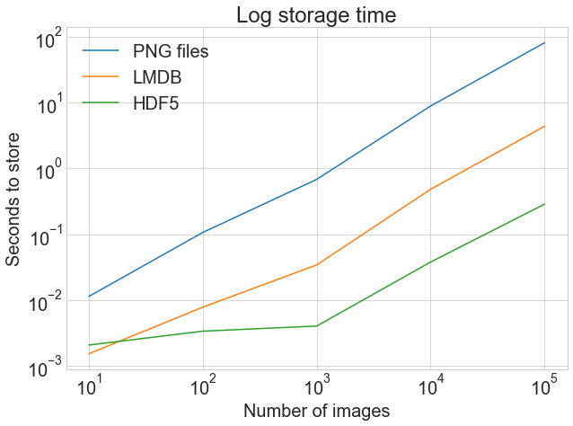
The first graph shows the normal, unadjusted storage time, highlighting the drastic difference between storing to .png files and LMDB or HDF5.
The second graph shows the log of the timings, highlighting that HDF5 starts out slower than LMDB but, with larger quantities of images, comes out slightly ahead.
While exact results may vary depending on your machine, this is why LMDB and HDF5 are worth thinking about. Here’s the code that generated the above graph:
import matplotlib.pyplot as plt

def plot_with_legend(
    x_range, y_data, legend_labels, x_label, y_label, title, log=False
):
    """ Displays a single plot with multiple datasets and matching legends.
        Parameters:
        --------------
        x_range         list of lists containing x data
        y_data          list of lists containing y values
        legend_labels   list of string legend labels
        x_label         x axis label
        y_label         y axis label
    """
    plt.style.use("seaborn-whitegrid")
    plt.figure(figsize=(10, 7))

    if len(y_data) != len(legend_labels):
        raise TypeError(
            "Error: number of data sets does not match number of labels."
        )

    all_plots = []
    for data, label in zip(y_data, legend_labels):
        if log:
            temp, = plt.loglog(x_range, data, label=label)
        else:
            temp, = plt.plot(x_range, data, label=label)
        all_plots.append(temp)

    plt.title(title)
    plt.xlabel(x_label)
    plt.ylabel(y_label)
    plt.legend(handles=all_plots)
    plt.show()

# Getting the store timings data to display
disk_x = store_many_timings["disk"]
lmdb_x = store_many_timings["lmdb"]
hdf5_x = store_many_timings["hdf5"]

plot_with_legend(
    cutoffs,
    [disk_x, lmdb_x, hdf5_x],
    ["PNG files", "LMDB", "HDF5"],
    "Number of images",
    "Seconds to store",
    "Storage time",
    log=False,
)

plot_with_legend(
    cutoffs,
    [disk_x, lmdb_x, hdf5_x],
    ["PNG files", "LMDB", "HDF5"],
    "Number of images",
    "Seconds to store",
    "Log storage time",
    log=True,
)
Now let’s go on to reading the images back out.
Reading a Single Image
First, let’s consider the case for reading a single image back into an array for each of the three methods.
Reading From Disk
Of the three methods, LMDB requires the most legwork when reading image files back out of memory, because of the serialization step. Let’s walk through these functions that read a single image out for each of the three storage formats.
First, read a single image and its meta from a .png and .csv file:
def read_single_disk(image_id):
    """ Stores a single image to disk.
        Parameters:
        ---------------
        image_id    integer unique ID for image

        Returns:
        ----------
        image       image array, (32, 32, 3) to be stored
        label       associated meta data, int label
    """
    image = np.array(Image.open(disk_dir / f"{image_id}.png"))

    with open(disk_dir / f"{image_id}.csv", "r") as csvfile:
        reader = csv.reader(
            csvfile, delimiter=" ", quotechar="|", quoting=csv.QUOTE_MINIMAL
        )
        label = int(next(reader)[0])

    return image, label
Reading From LMDB
Next, read the same image and meta from an LMDB by opening the environment and starting a read transaction:
 1def read_single_lmdb(image_id):
 2    """ Stores a single image to LMDB.
 3        Parameters:
 4        ---------------
 5        image_id    integer unique ID for image
 6
 7        Returns:
 8        ----------
 9        image       image array, (32, 32, 3) to be stored
10        label       associated meta data, int label
11    """
12    # Open the LMDB environment
13    env = lmdb.open(str(lmdb_dir / f"single_lmdb"), readonly=True)
14
15    # Start a new read transaction
16    with env.begin() as txn:
17        # Encode the key the same way as we stored it
18        data = txn.get(f"{image_id:08}".encode("ascii"))
19        # Remember it's a CIFAR_Image object that is loaded
20        cifar_image = pickle.loads(data)
21        # Retrieve the relevant bits
22        image = cifar_image.get_image()
23        label = cifar_image.label
24    env.close()
25
26    return image, label
Here are a couple points to not about the code snippet above:
- Line 13: The
readonly=Trueflag specifies that no writes will be allowed on the LMDB file until the transaction is finished. In database lingo, it’s equivalent to taking a read lock. - Line 20: To retrieve the CIFAR_Image object, you need to reverse the steps we took to pickle it when we were writing it. This is where the
get_image()of the object is helpful.
This wraps up reading the image back out from LMDB. Finally, you will want to do the same with HDF5.
Reading From HDF5
Reading from HDF5 looks very similar to the writing process. Here is the code to open and read the HDF5 file and parse the same image and meta:
def read_single_hdf5(image_id):
    """ Stores a single image to HDF5.
        Parameters:
        ---------------
        image_id    integer unique ID for image

        Returns:
        ----------
        image       image array, (32, 32, 3) to be stored
        label       associated meta data, int label
    """
    # Open the HDF5 file
    file = h5py.File(hdf5_dir / f"{image_id}.h5", "r+")

    image = np.array(file["/image"]).astype("uint8")
    label = int(np.array(file["/meta"]).astype("uint8"))

    return image, label
Note that you access the various datasets in the file by indexing the file object using the dataset name preceded by a forward slash /. As before, you can create a dictionary containing all the read functions:
_read_single_funcs = dict(
    disk=read_single_disk, lmdb=read_single_lmdb, hdf5=read_single_hdf5
)
With this dictionary prepared, you are ready for running the experiment.
Experiment for Reading a Single Image
You might expect that the experiment for reading a single image in will have somewhat trivial results, but here’s the experiment code:
from timeit import timeit

read_single_timings = dict()

for method in ("disk", "lmdb", "hdf5"):
    t = timeit(
        "_read_single_funcs[method](0)",
        setup="image=images[0]; label=labels[0]",
        number=1,
        globals=globals(),
    )
    read_single_timings[method] = t
    print(f"Method: {method}, Time usage: {t}")
Here are the results of the experiment for reading a single image:
| Method | Read Single Image + Meta |
|---|---|
| Disk | 1.61970 ms |
| LMDB | 4.52063 ms |
| HDF5 | 1.98036 ms |
It’s slightly faster to read the .png and .csv files directly from disk, but all three methods perform trivially quickly. The experiments we’ll do next are much more interesting.
Reading Many Images
Now you can adjust the code to read many images at once. This is likely the action you’ll be performing most often, so the runtime performance is essential.
Adjusting the Code for Many Images
Extending the functions above, you can create functions with read_many_, which can be used for the next experiments. Like before, it is interesting to compare performance when reading different quantities of images, which are repeated in the code below for reference:
def read_many_disk(num_images):
    """ Reads image from disk.
        Parameters:
        ---------------
        num_images   number of images to read

        Returns:
        ----------
        images      images array, (N, 32, 32, 3) to be stored
        labels      associated meta data, int label (N, 1)
    """
    images, labels = [], []

    # Loop over all IDs and read each image in one by one
    for image_id in range(num_images):
        images.append(np.array(Image.open(disk_dir / f"{image_id}.png")))

    with open(disk_dir / f"{num_images}.csv", "r") as csvfile:
        reader = csv.reader(
            csvfile, delimiter=" ", quotechar="|", quoting=csv.QUOTE_MINIMAL
        )
        for row in reader:
            labels.append(int(row[0]))
    return images, labels

def read_many_lmdb(num_images):
    """ Reads image from LMDB.
        Parameters:
        ---------------
        num_images   number of images to read

        Returns:
        ----------
        images      images array, (N, 32, 32, 3) to be stored
        labels      associated meta data, int label (N, 1)
    """
    images, labels = [], []
    env = lmdb.open(str(lmdb_dir / f"{num_images}_lmdb"), readonly=True)

    # Start a new read transaction
    with env.begin() as txn:
        # Read all images in one single transaction, with one lock
        # We could split this up into multiple transactions if needed
        for image_id in range(num_images):
            data = txn.get(f"{image_id:08}".encode("ascii"))
            # Remember that it's a CIFAR_Image object
            # that is stored as the value
            cifar_image = pickle.loads(data)
            # Retrieve the relevant bits
            images.append(cifar_image.get_image())
            labels.append(cifar_image.label)
    env.close()
    return images, labels

def read_many_hdf5(num_images):
    """ Reads image from HDF5.
        Parameters:
        ---------------
        num_images   number of images to read

        Returns:
        ----------
        images      images array, (N, 32, 32, 3) to be stored
        labels      associated meta data, int label (N, 1)
    """
    images, labels = [], []

    # Open the HDF5 file
    file = h5py.File(hdf5_dir / f"{num_images}_many.h5", "r+")

    images = np.array(file["/images"]).astype("uint8")
    labels = np.array(file["/meta"]).astype("uint8")

    return images, labels

_read_many_funcs = dict(
    disk=read_many_disk, lmdb=read_many_lmdb, hdf5=read_many_hdf5
)
With the reading functions stored in a dictionary as with the writing functions, you’re all set for the experiment.
Experiment for Reading Many Images
You can now run the experiment for reading many images out:
from timeit import timeit

read_many_timings = {"disk": [], "lmdb": [], "hdf5": []}

for cutoff in cutoffs:
    for method in ("disk", "lmdb", "hdf5"):
        t = timeit(
            "_read_many_funcs[method](num_images)",
            setup="num_images=cutoff",
            number=1,
            globals=globals(),
        )
        read_many_timings[method].append(t)

        # Print out the method, cutoff, and elapsed time
        print(f"Method: {method}, No. images: {cutoff}, Time usage: {t}")
As we did previously, you can graph the read experiment results:


The top graph shows the normal, unadjusted read times, showing the drastic difference between reading from .png files and LMDB or HDF5.
In contrast, the graph on the bottom shows the log of the timings, highlighting the relative differences with fewer images. Namely, we can see how HDF5 starts out behind but, with more images, becomes consistently faster than LMDB by a small margin.
Using the same plotting function as for the write timings, we have the following:
disk_x_r = read_many_timings["disk"]
lmdb_x_r = read_many_timings["lmdb"]
hdf5_x_r = read_many_timings["hdf5"]

plot_with_legend(
    cutoffs,
    [disk_x_r, lmdb_x_r, hdf5_x_r],
    ["PNG files", "LMDB", "HDF5"],
    "Number of images",
    "Seconds to read",
    "Read time",
    log=False,
)

plot_with_legend(
    cutoffs,
    [disk_x_r, lmdb_x_r, hdf5_x_r],
    ["PNG files", "LMDB", "HDF5"],
    "Number of images",
    "Seconds to read",
    "Log read time",
    log=True,
)
In practice, the write time is often less critical than the read time. Imagine that you are training a deep neural network on images, and only half of your entire image dataset fits into RAM at once. Each epoch of training a network requires the entire dataset, and the model needs a few hundred epochs to converge. You will essentially be reading half of the dataset into memory every epoch.
There are several tricks people do, such as training pseudo-epochs to make this slightly better, but you get the idea.
Now, look again at the read graph above. The difference between a 40-second and 4-second read time suddenly is the difference between waiting six hours for your model to train, or forty minutes!
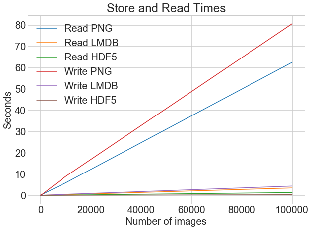
If we view the read and write times on the same chart, we have the following:
You can plot all the read and write timings on a single graph using the same plotting function:
plot_with_legend(
    cutoffs,
    [disk_x_r, lmdb_x_r, hdf5_x_r, disk_x, lmdb_x, hdf5_x],
    [
        "Read PNG",
        "Read LMDB",
        "Read HDF5",
        "Write PNG",
        "Write LMDB",
        "Write HDF5",
    ],
    "Number of images",
    "Seconds",
    "Log Store and Read Times",
    log=False,
)
When you’re storing images as .png files, there is a big difference between write and read times. However, with LMDB and HDF5, the difference is much less marked. Overall, even if read time is more critical than write time, there is a strong argument for storing images using LMDB or HDF5.
Now that you’ve seen the performance benefits of LMDB and HDF5, let’s look at another crucial metric: disk usage.
Considering Disk Usage
Speed is not the only performance metric you may be interested in. We’re already dealing with very large datasets, so disk space is also a very valid and relevant concern.
Suppose you have an image dataset of 3TB. Presumably, you have them already on disk somewhere, unlike our CIFAR example, so by using an alternate storage method, you are essentially making a copy of them, which also has to be stored. Doing so will give you huge performance benefits when you use the images, but you’ll need to make sure you have enough disk space.
How much disk space do the various storage methods use? Here’s the disk space used for each method for each quantity of images:
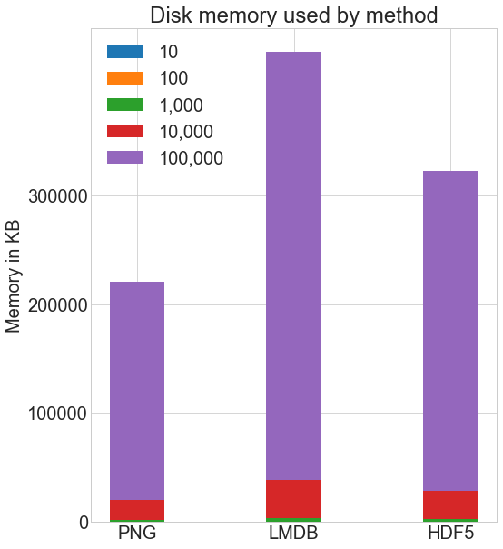
I used the Linux du -h -c folder_name/* command to compute the disk usage on my system. There is some approximation inherent with this method due to rounding, but here’s the general comparison:
# Memory used in KB
disk_mem = [24, 204, 2004, 20032, 200296]
lmdb_mem = [60, 420, 4000, 39000, 393000]
hdf5_mem = [36, 304, 2900, 29000, 293000]

X = [disk_mem, lmdb_mem, hdf5_mem]

ind = np.arange(3)
width = 0.35

plt.subplots(figsize=(8, 10))
plots = [plt.bar(ind, [row[0] for row in X], width)]
for i in range(1, len(cutoffs)):
    plots.append(
        plt.bar(
            ind, [row[i] for row in X], width, bottom=[row[i - 1] for row in X]
        )
    )

plt.ylabel("Memory in KB")
plt.title("Disk memory used by method")
plt.xticks(ind, ("PNG", "LMDB", "HDF5"))
plt.yticks(np.arange(0, 400000, 100000))

plt.legend(
    [plot[0] for plot in plots], ("10", "100", "1,000", "10,000", "100,000")
)
plt.show()
Both HDF5 and LMDB take up more disk space than if you store using normal .png images. It’s important to note that both LMDB and HDF5 disk usage and performance depend highly on various factors, including operating system and, more critically, the size of the data you store.
LMDB gains its efficiency from caching and taking advantage of OS page sizes. You don’t need to understand its inner workings, but note that with larger images, you will end up with significantly more disk usage with LMDB, because images won’t fit on LMDB’s leaf pages, the regular storage location in the tree, and instead you will have many overflow pages. The LMDB bar in the chart above will shoot off the chart.
Our 32x32x3 pixel images are relatively small compared to the average images you may use, and they allow for optimal LMDB performance.
While we won’t explore it here experimentally, in my own experience with images of 256x256x3 or 512x512x3 pixels, HDF5 is usually slightly more efficient in terms of disk usage than LMDB. This is a good transition into the final section, a qualitative discussion of the differences between the methods.
Discussion
There are other distinguishing features of LMDB and HDF5 that are worth knowing about, and it’s also important to briefly discuss some of the criticisms of both methods. Several links are included along with the discussion if you want to learn more.
Parallel Access
A key comparison that we didn’t test in the experiments above is concurrent reads and writes. Often, with such large datasets, you may want to speed up your operation through parallelization.
In the majority of cases, you won’t be interested in reading parts of the same image at the same time, but you will want to read multiple images at once. With this definition of concurrency, storing to disk as .png files actually allows for complete concurrency. Nothing prevents you from reading several images at once from different threads, or writing multiple files at once, as long as the image names are different.
How about LMDB? There can be multiple readers on an LMDB environment at a time, but only one writer, and writers do not block readers. You can read more about that at the LMDB technology website.
Multiple applications can access the same LMDB database at the same time, and multiple threads from the same process can also concurrently access the LMDB for reads. This allows for even quicker read times: if you divided all of CIFAR into ten sets, then you could set up ten processes to each read in one set, and it would divide the loading time by ten.
HDF5 also offers parallel I/O, allowing concurrent reads and writes. However, in implementation, a write lock is held, and access is sequential, unless you have a parallel file system.
There are two main options if you are working on such a system, which are discussed more in depth in this article by the HDF Group on parallel IO. It can get quite complicated, and the simplest option is to intelligently split your dataset into multiple HDF5 files, such that each process can deal with one .h5 file independently of the others.
Documentation
If you Google lmdb, at least in the United Kingdom, the third search result is IMDb, the Internet Movie Database. That’s not what you were looking for!
Actually, there is one main source of documentation for the Python binding of LMDB, which is hosted on Read the Docs LMDB. While the Python package hasn’t even reached version > 0.94, it is quite widely used and is considered stable.
As for the LMDB technology itself, there is more detailed documentation at the LMDB technology website, which can feel a bit like learning calculus in second grade, unless you start from their Getting Started page.
For HDF5, there is very clear documentation at the h5py docs site, as well as a helpful blog post by Christopher Lovell, which is an excellent overview of how to use the h5py package. The O’Reilly book, Python and HDF5 also is a good way to get started.
While not as documented as perhaps a beginner would appreciate, both LMDB and HDF5 have large user communities, so a deeper Google search usually yields helpful results.
A More Critical Look at Implementation
There is no utopia in storage systems, and both LMDB and HDF5 have their share of pitfalls.
A key point to understand about LMDB is that new data is written without overwriting or moving existing data. This is a design decision that allows for the extremely quick reads you witnessed in our experiments, and also guarantees data integrity and reliability without the additional need of keeping transaction logs.
Remember, however, that you needed to define the map_size parameter for memory allocation before writing to a new database? This is where LMDB can be a hassle. Suppose you have created an LMDB database, and everything is wonderful. You’ve waited patiently for your enormous dataset to be packed into a LMDB.
Then, later down the line, you remember that you need to add new data. Even with the buffer you specified on your map_size, you may easily expect to see the lmdb.MapFullError error. Unless you want to re-write your entire database, with the updated map_size, you’ll have to store that new data in a separate LMDB file. Even though one transaction can span multiple LMDB files, having multiple files can still be a pain.
Additionally, some systems have restrictions on how much memory may be claimed at once. In my own experience, working with high-performance computing (HPC) systems, this has proved extremely frustrating, and has often made me prefer HDF5 over LMDB.
With both LMDB and HDF5, only the requested item is read into memory at once. With LMDB, key-unit pairs are read into memory one by one, while with HDF5, the dataset object can be accessed like a Python array, with indexing dataset[i], ranges, dataset[i:j] and other splicing dataset[i:j:interval].
Because of the way the systems are optimized, and depending on your operating system, the order in which you access items can impact performance.
In my experience, it’s generally true that for LMDB, you may get better performance when accessing items sequentially by key (key-value pairs being kept in memory ordered alphanumerically by key), and that for HDF5, accessing large ranges will perform better than reading every element of the dataset one by one using the following:
# Slightly slower
for i in range(len(dataset)):
    # Read the ith value in the dataset, one at a time
    do_something_with(dataset[i])

# This is better
data = dataset[:]
for d in data:
    do_something_with(d)
If you are considering a choice of file storage format to write your software around, it would be remiss not to mention Moving away from HDF5 by Cyrille Rossant on the pitfalls of HDF5, and Konrad Hinsen’s response On HDF5 and the future of data management, which shows how some of the pitfalls can be avoided in his own use cases with many smaller datasets rather than a few enormous ones. Note that a relatively smaller dataset is still several GB in size.
Integration With Other Libraries
If you’re dealing with really large datasets, it’s highly likely that you’ll be doing something significant with them. It’s worthwhile to consider deep learning libraries and what kind of integration there is with LMDB and HDF5.
First of all, all libraries support reading images from disk as .png files, as long as you convert them into NumPy arrays of the expected format. This holds true for all the methods, and we have already seen above that it is relatively straightforward to read in images as arrays.
Here are several of the most popular deep learning libraries and their LMDB and HDF5 integration:
-
Caffe has a stable, well-supported LMDB integration, and it handles the reading step transparently. The LMDB layer can also easily be replaced with a HDF5 database.
-
Keras uses the HDF5 format to save and restore models. This implies that TensorFlow can as well.
-
TensorFlow has a built-in class
LMDBDatasetthat provides an interface for reading in input data from an LMDB file and can produce iterators and tensors in batches. TensorFlow does not have a built-in class for HDF5, but one can be written that inherits from theDatasetclass. I personally use a custom class altogether that is designed for optimal read access based on the way I structure my HDF5 files. -
Theano does not natively support any particular file format or database, but as previously stated, can use anything as long as it is read in as an N-dimensional array.
While far from comprehensive, this hopefully gives you a feel for the LMDB/HDF5 integration by some key deep learning libraries.
A Few Personal Insights on Storing Images in Python
In my own daily work analyzing terabytes of medical images, I use both LMDB and HDF5, and have learned that, with any storage method, forethought is critical.
Often, models need to be trained using k-fold cross validation, which involves splitting the entire dataset into k-sets (k typically being 10), and k models being trained, each with a different k-set used as test set. This ensures that the model is not overfitting the dataset, or, in other words, unable to make good predictions on unseen data.
A standard way to craft a k-set is to put an equal representation of each type of data represented in the dataset in each k-set. Thus, saving each k-set into a separate HDF5 dataset maximizes efficiency. Sometimes, a single k-set cannot be loaded into memory at once, so even the ordering of data within a dataset requires some forethought.
With LMDB, I similarly am careful to plan ahead before creating the database(s). There are a few good questions worth asking before you save images:
- How can I save the images such that most of the reads will be sequential?
- What are good keys?
- How can I calculate a good
map_size, anticipating potential future changes in the dataset? - How large can a single transaction be, and how should transactions be subdivided?
Regardless of the storage method, when you’re dealing with large image datasets, a little planning goes a long way.
Conclusion
You’ve made it to the end! You’ve now had a bird’s eye view of a large topic.
In this article, you’ve been introduced to three ways of storing and accessing lots of images in Python, and perhaps had a chance to play with some of them. All the code for this article is in a Jupyter notebook here or Python script here. Run at your own risk, as a few GB of your disk space will be overtaken by little square images of cars, boats, and so on.
You’ve seen evidence of how various storage methods can drastically affect read and write time, as well as a few pros and cons of the three methods considered in this article. While storing images as .png files may be the most intuitive, there are large performance benefits to considering methods such as HDF5 or LMDB.
Feel free to discuss in the comment section the excellent storage methods not covered in this article, such as LevelDB, Feather, TileDB, Badger, BoltDB, or anything else. There is no perfect storage method, and the best method depends on your specific dataset and use cases.
Further Reading
Here are some references related to the three methods covered in this article:
- Python binding for LMDB
- LMDB documentation: Getting Started
- Python binding for HDF5 (h5py)
- The HDF5 Group
- “Python and HDF5” from O’Reilly
- Pillow
You may also appreciate “An analysis of image storage systems for scalable training of deep neural networks” by Lim, Young, and Patton. That paper covers experiments similar to the ones in this article, but on a much larger scale, considering cold and warm cache as well as other factors.