Watch Now This tutorial has a related video course created by the Real Python team. Watch it together with the written tutorial to deepen your understanding: Building a Neural Network & Making Predictions With Python AI
If you’re just starting out in the artificial intelligence (AI) world, then Python is a great language to learn since most of the tools are built using it. Deep learning is a technique used to make predictions using data, and it heavily relies on neural networks. Today, you’ll learn how to build a neural network from scratch.
In a production setting, you would use a deep learning framework like TensorFlow or PyTorch instead of building your own neural network. That said, having some knowledge of how neural networks work is helpful because you can use it to better architect your deep learning models.
In this tutorial, you’ll learn:
- What artificial intelligence is
- How both machine learning and deep learning play a role in AI
- How a neural network functions internally
- How to build a neural network from scratch using Python
Let’s get started!
Free Bonus: Click here to get access to a free NumPy Resources Guide that points you to the best tutorials, videos, and books for improving your NumPy skills.
Artificial Intelligence Overview
In basic terms, the goal of using AI is to make computers think as humans do. This may seem like something new, but the field was born in the 1950s.
Imagine that you need to write a Python program that uses AI to solve a sudoku problem. A way to accomplish that is to write conditional statements and check the constraints to see if you can place a number in each position. Well, this Python script is already an application of AI because you programmed a computer to solve a problem!
Machine learning (ML) and deep learning (DL) are also approaches to solving problems. The difference between these techniques and a Python script is that ML and DL use training data instead of hard-coded rules, but all of them can be used to solve problems using AI. In the next sections, you’ll learn more about what differentiates these two techniques.
Machine Learning
Machine learning is a technique in which you train the system to solve a problem instead of explicitly programming the rules. Getting back to the sudoku example in the previous section, to solve the problem using machine learning, you would gather data from solved sudoku games and train a statistical model. Statistical models are mathematically formalized ways to approximate the behavior of a phenomenon.
A common machine learning task is supervised learning, in which you have a dataset with inputs and known outputs. The task is to use this dataset to train a model that predicts the correct outputs based on the inputs. The image below presents the workflow to train a model using supervised learning:
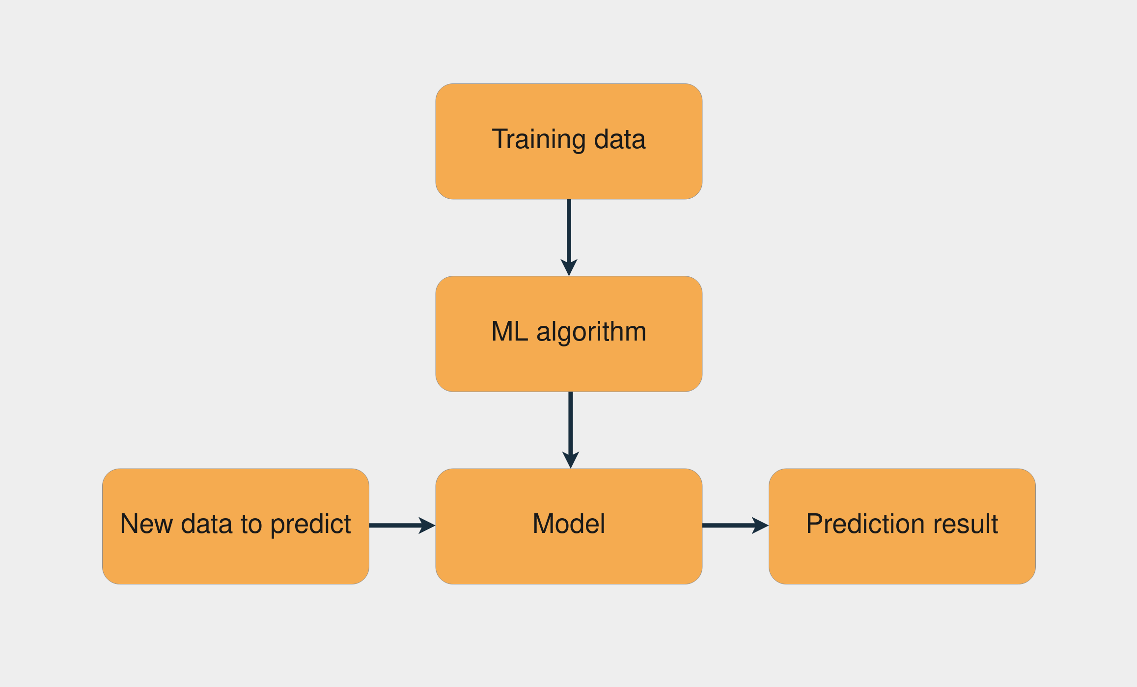
The combination of the training data with the machine learning algorithm creates the model. Then, with this model, you can make predictions for new data.
Note: scikit-learn is a popular Python machine learning library that provides many supervised and unsupervised learning algorithms. To learn more about it, check out Split Your Dataset With scikit-learn’s train_test_split().
The goal of supervised learning tasks is to make predictions for new, unseen data. To do that, you assume that this unseen data follows a probability distribution similar to the distribution of the training dataset. If in the future this distribution changes, then you need to train your model again using the new training dataset.
Feature Engineering
Prediction problems become harder when you use different kinds of data as inputs. The sudoku problem is relatively straightforward because you’re dealing directly with numbers. What if you want to train a model to predict the sentiment in a sentence? Or what if you have an image, and you want to know whether it depicts a cat?
Another name for input data is feature, and feature engineering is the process of extracting features from raw data. When dealing with different kinds of data, you need to figure out ways to represent this data in order to extract meaningful information from it.
An example of a feature engineering technique is lemmatization, in which you remove the inflection from words in a sentence. For example, inflected forms of the verb “watch,” like “watches,” “watching,” and “watched,” would be reduced to their lemma, or base form: “watch.”
If you’re using arrays to store each word of a corpus, then by applying lemmatization, you end up with a less-sparse matrix. This can increase the performance of some machine learning algorithms. The following image presents the process of lemmatization and representation using a bag-of-words model:

First, the inflected form of every word is reduced to its lemma. Then, the number of occurrences of that word is computed. The result is an array containing the number of occurrences of every word in the text.
Deep Learning
Deep learning is a technique in which you let the neural network figure out by itself which features are important instead of applying feature engineering techniques. This means that, with deep learning, you can bypass the feature engineering process.
Not having to deal with feature engineering is good because the process gets harder as the datasets become more complex. For example, how would you extract the data to predict the mood of a person given a picture of her face? With neural networks, you don’t need to worry about it because the networks can learn the features by themselves. In the next sections, you’ll dive deep into neural networks to better understand how they work.
Neural Networks: Main Concepts
A neural network is a system that learns how to make predictions by following these steps:
- Taking the input data
- Making a prediction
- Comparing the prediction to the desired output
- Adjusting its internal state to predict correctly the next time
Vectors, layers, and linear regression are some of the building blocks of neural networks. The data is stored as vectors, and with Python you store these vectors in arrays. Each layer transforms the data that comes from the previous layer. You can think of each layer as a feature engineering step, because each layer extracts some representation of the data that came previously.
One cool thing about neural network layers is that the same computations can extract information from any kind of data. This means that it doesn’t matter if you’re using image data or text data. The process to extract meaningful information and train the deep learning model is the same for both scenarios.
In the image below, you can see an example of a network architecture with two layers:

Each layer transforms the data that came from the previous layer by applying some mathematical operations.
The Process to Train a Neural Network
Training a neural network is similar to the process of trial and error. Imagine you’re playing darts for the first time. In your first throw, you try to hit the central point of the dartboard. Usually, the first shot is just to get a sense of how the height and speed of your hand affect the result. If you see the dart is higher than the central point, then you adjust your hand to throw it a little lower, and so on.
These are the steps for trying to hit the center of a dartboard:
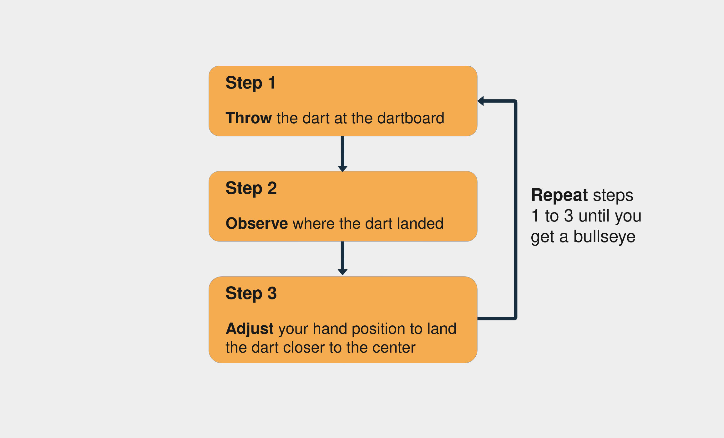
Notice that you keep assessing the error by observing where the dart landed (step 2). You go on until you finally hit the center of the dartboard.
With neural networks, the process is very similar: you start with some random weights and bias vectors, make a prediction, compare it to the desired output, and adjust the vectors to predict more accurately the next time. The process continues until the difference between the prediction and the correct targets is minimal.
Knowing when to stop the training and what accuracy target to set is an important aspect of training neural networks, mainly because of overfitting and underfitting scenarios.
Vectors and Weights
Working with neural networks consists of doing operations with vectors. You represent the vectors as multidimensional arrays. Vectors are useful in deep learning mainly because of one particular operation: the dot product. The dot product of two vectors tells you how similar they are in terms of direction and is scaled by the magnitude of the two vectors.
The main vectors inside a neural network are the weights and bias vectors. Loosely, what you want your neural network to do is to check if an input is similar to other inputs it’s already seen. If the new input is similar to previously seen inputs, then the outputs will also be similar. That’s how you get the result of a prediction.
The Linear Regression Model
Regression is used when you need to estimate the relationship between a dependent variable and two or more independent variables. Linear regression is a method applied when you approximate the relationship between the variables as linear. The method dates back to the nineteenth century and is the most popular regression method.
Note: A linear relationship is one where there’s a direct relationship between an independent variable and a dependent variable.
By modeling the relationship between the variables as linear, you can express the dependent variable as a weighted sum of the independent variables. So, each independent variable will be multiplied by a vector called weight. Besides the weights and the independent variables, you also add another vector: the bias. It sets the result when all the other independent variables are equal to zero.
As a real-world example of how to build a linear regression model, imagine you want to train a model to predict the price of houses based on the area and how old the house is. You decide to model this relationship using linear regression. The following code block shows how you can write a linear regression model for the stated problem in pseudocode:
price = (weights_area * area) + (weights_age * age) + bias
In the above example, there are two weights: weights_area and weights_age. The training process consists of adjusting the weights and the bias so the model can predict the correct price value. To accomplish that, you’ll need to compute the prediction error and update the weights accordingly.
These are the basics of how the neural network mechanism works. Now it’s time to see how to apply these concepts using Python.
Python AI: Starting to Build Your First Neural Network
The first step in building a neural network is generating an output from input data. You’ll do that by creating a weighted sum of the variables. The first thing you’ll need to do is represent the inputs with Python and NumPy.
Wrapping the Inputs of the Neural Network With NumPy
You’ll use NumPy to represent the input vectors of the network as arrays. But before you use NumPy, it’s a good idea to play with the vectors in pure Python to better understand what’s going on.
In this first example, you have an input vector and the other two weight vectors. The goal is to find which of the weights is more similar to the input, taking into account the direction and the magnitude. This is how the vectors look if you plot them:

weights_2 is more similar to the input vector since it’s pointing in the same direction and the magnitude is also similar. So how do you figure out which vectors are similar using Python?
First, you define the three vectors, one for the input and the other two for the weights. Then you compute how similar input_vector and weights_1 are. To do that, you’ll apply the dot product. Since all the vectors are two-dimensional vectors, these are the steps to do it:
- Multiply the first index of
input_vectorby the first index ofweights_1. - Multiply the second index of
input_vectorby the second index ofweights_2. - Sum the results of both multiplications.
You can use an IPython console or a Jupyter Notebook to follow along. It’s a good practice to create a new virtual environment every time you start a new Python project, so you should do that first. venv ships with Python versions 3.3 and above, and it’s handy for creating a virtual environment:
$ python -m venv ~/.my-env
$ source ~/.my-env/bin/activate
Using the above commands, you first create the virtual environment, then you activate it. Now it’s time to install the IPython console using pip. Since you’ll also need NumPy and Matplotlib, it’s a good idea install them too:
(my-env) $ python -m pip install ipython numpy matplotlib
(my-env) $ ipython
Now you’re ready to start coding. This is the code for computing the dot product of input_vector and weights_1:
In [1]: input_vector = [1.72, 1.23]
In [2]: weights_1 = [1.26, 0]
In [3]: weights_2 = [2.17, 0.32]

In [4]: # Computing the dot product of input_vector and weights_1
In [5]: first_indexes_mult = input_vector[0] * weights_1[0]
In [6]: second_indexes_mult = input_vector[1] * weights_1[1]
In [7]: dot_product_1 = first_indexes_mult + second_indexes_mult

In [8]: print(f"The dot product is: {dot_product_1}")
Out[8]: The dot product is: 2.1672
The result of the dot product is 2.1672. Now that you know how to compute the dot product, it’s time to use np.dot() from NumPy. Here’s how to compute dot_product_1 using np.dot():
In [9]: import numpy as np

In [10]: dot_product_1 = np.dot(input_vector, weights_1)

In [11]: print(f"The dot product is: {dot_product_1}")
Out[11]: The dot product is: 2.1672
np.dot() does the same thing you did before, but now you just need to specify the two arrays as arguments. Now let’s compute the dot product of input_vector and weights_2:
In [10]: dot_product_2 = np.dot(input_vector, weights_2)

In [11]: print(f"The dot product is: {dot_product_2}")
Out[11]: The dot product is: 4.1259
This time, the result is 4.1259. As a different way of thinking about the dot product, you can treat the similarity between the vector coordinates as an on-off switch. If the multiplication result is 0, then you’ll say that the coordinates are not similar. If the result is something other than 0, then you’ll say that they are similar.
This way, you can view the dot product as a loose measurement of similarity between the vectors. Every time the multiplication result is 0, the final dot product will have a lower result. Getting back to the vectors of the example, since the dot product of input_vector and weights_2 is 4.1259, and 4.1259 is greater than 2.1672, it means that input_vector is more similar to weights_2. You’ll use this same mechanism in your neural network.
Note: Click the prompt (>>>) at the top right of each code block if you need to copy and paste it.
In this tutorial, you’ll train a model to make predictions that have only two possible outcomes. The output result can be either 0 or 1. This is a classification problem, a subset of supervised learning problems in which you have a dataset with the inputs and the known targets. These are the inputs and the outputs of the dataset:
| Input Vector | Target |
|---|---|
| [1.66, 1.56] | 1 |
| [2, 1.5] | 0 |
The target is the variable you want to predict. In this example, you’re dealing with a dataset that consists of numbers. This isn’t common in a real production scenario. Usually, when there’s a need for a deep learning model, the data is presented in files, such as images or text.
Making Your First Prediction
Since this is your very first neural network, you’ll keep things straightforward and build a network with only two layers. So far, you’ve seen that the only two operations used inside the neural network were the dot product and a sum. Both are linear operations.
If you add more layers but keep using only linear operations, then adding more layers would have no effect because each layer will always have some correlation with the input of the previous layer. This implies that, for a network with multiple layers, there would always be a network with fewer layers that predicts the same results.
What you want is to find an operation that makes the middle layers sometimes correlate with an input and sometimes not correlate.
You can achieve this behavior by using nonlinear functions. These nonlinear functions are called activation functions. There are many types of activation functions. The ReLU (rectified linear unit), for example, is a function that converts all negative numbers to zero. This means that the network can “turn off” a weight if it’s negative, adding nonlinearity.
The network you’re building will use the sigmoid activation function. You’ll use it in the last layer, layer_2. The only two possible outputs in the dataset are 0 and 1, and the sigmoid function limits the output to a range between 0 and 1. This is the formula to express the sigmoid function:

The e is a mathematical constant called Euler’s number, and you can use np.exp(x) to calculate eˣ.
Probability functions give you the probability of occurrence for possible outcomes of an event. The only two possible outputs of the dataset are 0 and 1, and the Bernoulli distribution is a distribution that has two possible outcomes as well. The sigmoid function is a good choice if your problem follows the Bernoulli distribution, so that’s why you’re using it in the last layer of your neural network.
Since the function limits the output to a range of 0 to 1, you’ll use it to predict probabilities. If the output is greater than 0.5, then you’ll say the prediction is 1. If it’s below 0.5, then you’ll say the prediction is 0. This is the flow of the computations inside the network you’re building:

The yellow hexagons represent the functions, and the blue rectangles represent the intermediate results. Now it’s time to turn all this knowledge into code. You’ll also need to wrap the vectors with NumPy arrays. This is the code that applies the functions presented in the image above:
In [12]: # Wrapping the vectors in NumPy arrays
In [13]: input_vector = np.array([1.66, 1.56])
In [14]: weights_1 = np.array([1.45, -0.66])
In [15]: bias = np.array([0.0])

In [16]: def sigmoid(x):
   ...:     return 1 / (1 + np.exp(-x))

In [17]: def make_prediction(input_vector, weights, bias):
   ...:      layer_1 = np.dot(input_vector, weights) + bias
   ...:      layer_2 = sigmoid(layer_1)
   ...:      return layer_2

In [18]: prediction = make_prediction(input_vector, weights_1, bias)

In [19]: print(f"The prediction result is: {prediction}")
Out[19]: The prediction result is: [0.7985731]
The raw prediction result is 0.79, which is higher than 0.5, so the output is 1. The network made a correct prediction. Now try it with another input vector, np.array([2, 1.5]). The correct result for this input is 0. You’ll only need to change the input_vector variable since all the other parameters remain the same:
In [20]: # Changing the value of input_vector
In [21]: input_vector = np.array([2, 1.5])

In [22]: prediction = make_prediction(input_vector, weights_1, bias)

In [23]: print(f"The prediction result is: {prediction}")
Out[23]: The prediction result is: [0.87101915]
This time, the network made a wrong prediction. The result should be less than 0.5 since the target for this input is 0, but the raw result was 0.87. It made a wrong guess, but how bad was the mistake? The next step is to find a way to assess that.
Train Your First Neural Network
In the process of training the neural network, you first assess the error and then adjust the weights accordingly. To adjust the weights, you’ll use the gradient descent and backpropagation algorithms. Gradient descent is applied to find the direction and the rate to update the parameters.
Before making any changes in the network, you need to compute the error. That’s what you’ll do in the next section.
Computing the Prediction Error
To understand the magnitude of the error, you need to choose a way to measure it. The function used to measure the error is called the cost function, or loss function. In this tutorial, you’ll use the mean squared error (MSE) as your cost function. You compute the MSE in two steps:
- Compute the difference between the prediction and the target.
- Multiply the result by itself.
The network can make a mistake by outputting a value that’s higher or lower than the correct value. Since the MSE is the squared difference between the prediction and the correct result, with this metric you’ll always end up with a positive value.
This is the complete expression to compute the error for the last previous prediction:
In [24]: target = 0

In [25]: mse = np.square(prediction - target)

In [26]: print(f"Prediction: {prediction}; Error: {mse}")
Out[26]: Prediction: [0.87101915]; Error: [0.7586743596667225]
In the example above, the error is 0.75. One implication of multiplying the difference by itself is that bigger errors have an even larger impact, and smaller errors keep getting smaller as they decrease.
Understanding How to Reduce the Error
The goal is to change the weights and bias variables so you can reduce the error. To understand how this works, you’ll change only the weights variable and leave the bias fixed for now. You can also get rid of the sigmoid function and use only the result of layer_1. All that’s left is to figure out how you can modify the weights so that the error goes down.
You compute the MSE by doing error = np.square(prediction - target). If you treat (prediction - target) as a single variable x, then you have error = np.square(x), which is a quadratic function. Here’s how the function looks if you plot it:

The error is given by the y-axis. If you’re in point A and want to reduce the error toward 0, then you need to bring the x value down. On the other hand, if you’re in point B and want to reduce the error, then you need to bring the x value up. To know which direction you should go to reduce the error, you’ll use the derivative. A derivative explains exactly how a pattern will change.
Another word for the derivative is gradient. Gradient descent is the name of the algorithm used to find the direction and the rate to update the network parameters.
Note: To learn more about the math behind gradient descent, check out Stochastic Gradient Descent Algorithm With Python and NumPy.
In this tutorial, you won’t focus on the theory behind derivatives, so you’ll simply apply the derivative rules for each function you’ll encounter. The power rule states that the derivative of xⁿ is nx⁽ⁿ⁻¹⁾. So the derivative of np.square(x) is 2 * x, and the derivative of x is 1.
Remember that the error expression is error = np.square(prediction - target). When you treat (prediction - target) as a single variable x, the derivative of the error is 2 * x. By taking the derivative of this function, you want to know in what direction should you change x to bring the result of error to zero, thereby reducing the error.
When it comes to your neural network, the derivative will tell you the direction you should take to update the weights variable. If it’s a positive number, then you predicted too high, and you need to decrease the weights. If it’s a negative number, then you predicted too low, and you need to increase the weights.
Now it’s time to write the code to figure out how to update weights_1 for the previous wrong prediction. If the mean squared error is 0.75, then should you increase or decrease the weights? Since the derivative is 2 * x, you just need to multiply the difference between the prediction and the target by 2:
In [27]: derivative = 2 * (prediction - target)

In [28]: print(f"The derivative is {derivative}")
Out[28]: The derivative is: [1.7420383]
The result is 1.74, a positive number, so you need to decrease the weights. You do that by subtracting the derivative result of the weights vector. Now you can update weights_1 accordingly and predict again to see how it affects the prediction result:
In [29]: # Updating the weights
In [30]: weights_1 = weights_1 - derivative

In [31]: prediction = make_prediction(input_vector, weights_1, bias)

In [32]: error = (prediction - target) ** 2

In [33]: print(f"Prediction: {prediction}; Error: {error}")
Out[33]: Prediction: [0.01496248]; Error: [0.00022388]
The error dropped down to almost 0! Beautiful, right? In this example, the derivative result was small, but there are some cases where the derivative result is too high. Take the image of the quadratic function as an example. High increments aren’t ideal because you could keep going from point A straight to point B, never getting close to zero. To cope with that, you update the weights with a fraction of the derivative result.
To define a fraction for updating the weights, you use the alpha parameter, also called the learning rate. If you decrease the learning rate, then the increments are smaller. If you increase it, then the steps are higher. How do you know what’s the best learning rate value? By making a guess and experimenting with it.
Note: Traditional default learning rate values are 0.1, 0.01, and 0.001.
If you take the new weights and make a prediction with the first input vector, then you’ll see that now it makes a wrong prediction for that one. If your neural network makes a correct prediction for every instance in your training set, then you probably have an overfitted model, where the model simply remembers how to classify the examples instead of learning to notice features in the data.
There are techniques to avoid that, including regularization the stochastic gradient descent. In this tutorial you’ll use the online stochastic gradient descent.
Now that you know how to compute the error and how to adjust the weights accordingly, it’s time to get back continue building your neural network.
Applying the Chain Rule
In your neural network, you need to update both the weights and the bias vectors. The function you’re using to measure the error depends on two independent variables, the weights and the bias. Since the weights and the bias are independent variables, you can change and adjust them to get the result you want.
The network you’re building has two layers, and since each layer has its own functions, you’re dealing with a function composition. This means that the error function is still np.square(x), but now x is the result of another function.
To restate the problem, now you want to know how to change weights_1 and bias to reduce the error. You already saw that you can use derivatives for this, but instead of a function with only a sum inside, now you have a function that produces its result using other functions.
Since now you have this function composition, to take the derivative of the error concerning the parameters, you’ll need to use the chain rule from calculus. With the chain rule, you take the partial derivatives of each function, evaluate them, and multiply all the partial derivatives to get the derivative you want.
Now you can start updating the weights. You want to know how to change the weights to decrease the error. This implies that you need to compute the derivative of the error with respect to weights. Since the error is computed by combining different functions, you need to take the partial derivatives of these functions.
Here’s a visual representation of how you apply the chain rule to find the derivative of the error with respect to the weights:

The bold red arrow shows the derivative you want, derror_dweights. You’ll start from the red hexagon, taking the inverse path of making a prediction and computing the partial derivatives at each function.
In the image above, each function is represented by the yellow hexagons, and the partial derivatives are represented by the gray arrows on the left. Applying the chain rule, the value of derror_dweights will be the following:
derror_dweights = (
    derror_dprediction * dprediction_dlayer1 * dlayer1_dweights
)
To calculate the derivative, you multiply all the partial derivatives that follow the path from the error hexagon (the red one) to the hexagon where you find the weights (the leftmost green one).
You can say that the derivative of y = f(x) is the derivative of f with respect to x. Using this nomenclature, for derror_dprediction, you want to know the derivative of the function that computes the error with respect to the prediction value.
This reverse path is called a backward pass. In each backward pass, you compute the partial derivatives of each function, substitute the variables by their values, and finally multiply everything.
This “take the partial derivatives, evaluate, and multiply” part is how you apply the chain rule. This algorithm to update the neural network parameters is called backpropagation.
Adjusting the Parameters With Backpropagation
In this section, you’ll walk through the backpropagation process step by step, starting with how you update the bias. You want to take the derivative of the error function with respect to the bias, derror_dbias. Then you’ll keep going backward, taking the partial derivatives until you find the bias variable.
Since you are starting from the end and going backward, you first need to take the partial derivative of the error with respect to the prediction. That’s the derror_dprediction in the image below:

The function that produces the error is a square function, and the derivative of this function is 2 * x, as you saw earlier. You applied the first partial derivative (derror_dprediction) and still didn’t get to the bias, so you need to take another step back and take the derivative of the prediction with respect to the previous layer, dprediction_dlayer1.
The prediction is the result of the sigmoid function. You can take the derivative of the sigmoid function by multiplying sigmoid(x) and 1 - sigmoid(x). This derivative formula is very handy because you can use the sigmoid result that has already been computed to compute the derivative of it. You then take this partial derivative and continue going backward.
Now you’ll take the derivative of layer_1 with respect to the bias. There it is—you finally got to it! The bias variable is an independent variable, so the result after applying the power rule is 1. Cool, now that you’ve completed this backward pass, you can put everything together and compute derror_dbias:
In [36]: def sigmoid_deriv(x):
   ...:     return sigmoid(x) * (1-sigmoid(x))

In [37]: derror_dprediction = 2 * (prediction - target)
In [38]: layer_1 = np.dot(input_vector, weights_1) + bias
In [39]: dprediction_dlayer1 = sigmoid_deriv(layer_1)
In [40]: dlayer1_dbias = 1

In [41]: derror_dbias = (
   ...:     derror_dprediction * dprediction_dlayer1 * dlayer1_dbias
   ...: )
To update the weights, you follow the same process, going backward and taking the partial derivatives until you get to the weights variable. Since you’ve already computed some of the partial derivatives, you’ll just need to compute dlayer1_dweights. The derivative of the dot product is the derivative of the first vector multiplied by the second vector, plus the derivative of the second vector multiplied by the first vector.
Creating the Neural Network Class
Now you know how to write the expressions to update both the weights and the bias. It’s time to create a class for the neural network. Classes are the main building blocks of object-oriented programming (OOP). The NeuralNetwork class generates random start values for the weights and bias variables.
When instantiating a NeuralNetwork object, you need to pass the learning_rate parameter. You’ll use predict() to make a prediction. The methods _compute_derivatives() and _update_parameters() have the computations you learned in this section. This is the final NeuralNetwork class:
class NeuralNetwork:
    def __init__(self, learning_rate):
        self.weights = np.array([np.random.randn(), np.random.randn()])
        self.bias = np.random.randn()
        self.learning_rate = learning_rate

    def _sigmoid(self, x):
        return 1 / (1 + np.exp(-x))

    def _sigmoid_deriv(self, x):
        return self._sigmoid(x) * (1 - self._sigmoid(x))

    def predict(self, input_vector):
        layer_1 = np.dot(input_vector, self.weights) + self.bias
        layer_2 = self._sigmoid(layer_1)
        prediction = layer_2
        return prediction

    def _compute_gradients(self, input_vector, target):
        layer_1 = np.dot(input_vector, self.weights) + self.bias
        layer_2 = self._sigmoid(layer_1)
        prediction = layer_2

        derror_dprediction = 2 * (prediction - target)
        dprediction_dlayer1 = self._sigmoid_deriv(layer_1)
        dlayer1_dbias = 1
        dlayer1_dweights = (0 * self.weights) + (1 * input_vector)

        derror_dbias = (
            derror_dprediction * dprediction_dlayer1 * dlayer1_dbias
        )
        derror_dweights = (
            derror_dprediction * dprediction_dlayer1 * dlayer1_dweights
        )

        return derror_dbias, derror_dweights

    def _update_parameters(self, derror_dbias, derror_dweights):
        self.bias = self.bias - (derror_dbias * self.learning_rate)
        self.weights = self.weights - (
            derror_dweights * self.learning_rate
        )
There you have it: That’s the code of your first neural network. Congratulations! This code just puts together all the pieces you’ve seen so far. If you want to make a prediction, first you create an instance of NeuralNetwork(), and then you call .predict():
In [42]: learning_rate = 0.1

In [43]: neural_network = NeuralNetwork(learning_rate)

In [44]: neural_network.predict(input_vector)
Out[44]: array([0.79412963])
The above code makes a prediction, but now you need to learn how to train the network. The goal is to make the network generalize over the training dataset. This means that you want it to adapt to new, unseen data that follow the same probability distribution as the training dataset. That’s what you’ll do in the next section.
Training the Network With More Data
You’ve already adjusted the weights and the bias for one data instance, but the goal is to make the network generalize over an entire dataset. Stochastic gradient descent is a technique in which, at every iteration, the model makes a prediction based on a randomly selected piece of training data, calculates the error, and updates the parameters.
Now it’s time to create the train() method of your NeuralNetwork class. You’ll save the error over all data points every 100 iterations because you want to plot a chart showing how this metric changes as the number of iterations increases. This is the final train() method of your neural network:
 1class NeuralNetwork:
 2    # ...
 3
 4    def train(self, input_vectors, targets, iterations):
 5        cumulative_errors = []
 6        for current_iteration in range(iterations):
 7            # Pick a data instance at random
 8            random_data_index = np.random.randint(len(input_vectors))
 9
10            input_vector = input_vectors[random_data_index]
11            target = targets[random_data_index]
12
13            # Compute the gradients and update the weights
14            derror_dbias, derror_dweights = self._compute_gradients(
15                input_vector, target
16            )
17
18            self._update_parameters(derror_dbias, derror_dweights)
19
20            # Measure the cumulative error for all the instances
21            if current_iteration % 100 == 0:
22                cumulative_error = 0
23                # Loop through all the instances to measure the error
24                for data_instance_index in range(len(input_vectors)):
25                    data_point = input_vectors[data_instance_index]
26                    target = targets[data_instance_index]
27
28                    prediction = self.predict(data_point)
29                    error = np.square(prediction - target)
30
31                    cumulative_error = cumulative_error + error
32                cumulative_errors.append(cumulative_error)
33
34        return cumulative_errors
There’s a lot going on in the above code block, so here’s a line-by-line breakdown:
-
Line 8 picks a random instance from the dataset.
-
Lines 14 to 16 calculate the partial derivatives and return the derivatives for the bias and the weights. They use
_compute_gradients(), which you defined earlier. -
Line 18 updates the bias and the weights using
_update_parameters(), which you defined in the previous code block. -
Line 21 checks if the current iteration index is a multiple of
100. You do this to observe how the error changes every100iterations. -
Line 24 starts the loop that goes through all the data instances.
-
Line 28 computes the
predictionresult. -
Line 29 computes the
errorfor every instance. -
Line 31 is where you accumulate the sum of the errors using the
cumulative_errorvariable. You do this because you want to plot a point with the error for all the data instances. Then, on line 32, you append theerrortocumulative_errors, the array that stores the errors. You’ll use this array to plot the graph.
In short, you pick a random instance from the dataset, compute the gradients, and update the weights and the bias. You also compute the cumulative error every 100 iterations and save those results in an array. You’ll plot this array to visualize how the error changes during the training process.
Note: If you’re running the code in a Jupyter Notebook, then you need to restart the kernel after adding train() to the NeuralNetwork class.
To keep things less complicated, you’ll use a dataset with just eight instances, the input_vectors array. Now you can call train() and use Matplotlib to plot the cumulative error for each iteration:
In [45]: # Paste the NeuralNetwork class code here
   ...: # (and don't forget to add the train method to the class)

In [46]: import matplotlib.pyplot as plt

In [47]: input_vectors = np.array(
   ...:     [
   ...:         [3, 1.5],
   ...:         [2, 1],
   ...:         [4, 1.5],
   ...:         [3, 4],
   ...:         [3.5, 0.5],
   ...:         [2, 0.5],
   ...:         [5.5, 1],
   ...:         [1, 1],
   ...:     ]
   ...: )

In [48]: targets = np.array([0, 1, 0, 1, 0, 1, 1, 0])

In [49]: learning_rate = 0.1

In [50]: neural_network = NeuralNetwork(learning_rate)

In [51]: training_error = neural_network.train(input_vectors, targets, 10000)

In [52]: plt.plot(training_error)
In [53]: plt.xlabel("Iterations")
In [54]: plt.ylabel("Error for all training instances")
In [54]: plt.savefig("cumulative_error.png")
You instantiate the NeuralNetwork class again and call train() using the input_vectors and the target values. You specify that it should run 10000 times. This is the graph showing the error for an instance of a neural network:

The overall error is decreasing, which is what you want. The image is generated in the same directory where you’re running IPython. After the largest decrease, the error keeps going up and down quickly from one interaction to another. That’s because the dataset is random and very small, so it’s hard for the neural network to extract any features.
But it’s not a good idea to evaluate the performance using this metric because you’re evaluating it using data instances that the network already saw. This can lead to overfitting, when the model fits the training dataset so well that it doesn’t generalize to new data.
Adding More Layers to the Neural Network
The dataset in this tutorial was kept small for learning purposes. Usually, deep learning models need a large amount of data because the datasets are more complex and have a lot of nuances.
Since these datasets have more complex information, using only one or two layers isn’t enough. That’s why deep learning models are called “deep.” They usually have a large number of layers.
By adding more layers and using activation functions, you increase the network’s expressive power and can make very high-level predictions. An example of these types of predictions is face recognition, such as when you take a photo of your face with your phone, and the phone unlocks if it recognizes the image as you.
Conclusion
Congratulations! Today, you built a neural network from scratch using NumPy. With this knowledge, you’re ready to dive deeper into the world of artificial intelligence in Python.
In this tutorial, you learned:
- What deep learning is and what differentiates it from machine learning
- How to represent vectors with NumPy
- What activation functions are and why they’re used inside a neural network
- What the backpropagation algorithm is and how it works
- How to train a neural network and make predictions
The process of training a neural network mainly consists of applying operations to vectors. Today, you did it from scratch using only NumPy as a dependency. This isn’t recommended in a production setting because the whole process can be unproductive and error-prone. That’s one of the reasons why deep learning frameworks like Keras, PyTorch, and TensorFlow are so popular.
Further Reading
For additional information on topics covered in this tutorial, check out these resources:
Watch Now This tutorial has a related video course created by the Real Python team. Watch it together with the written tutorial to deepen your understanding: Building a Neural Network & Making Predictions With Python AI